Getting Good Images

This section covers techniques for getting good astro-images using the features available in SharpCap. In particular, use of the Histogram and Smart Histogram functions help set the correct exposure and gain for your camera and the type of image being captured. The focus assistance tools – ranging from just measuring the quality of focus to full autofocus will help ensure that you capture sharp images.

Correctly Exposing Images using the Histogram

The Histogram

The image histogram acts as a graphical representation of the brightness distribution in a digital image.  It plots the number of pixels for each brightness value.  The histogram will quickly highlight problems with an image including under exposure, over exposure or colour balance issues and is used to help capture the highest quality data possible.

The histogram can be shown by clicking the Image Histogram icon in the Tool Bar:

which will display the Image Histogram in the Work Area of the Main Screen, as shown below.

c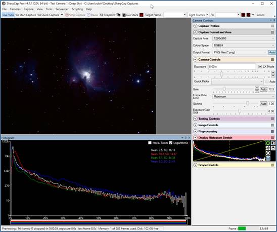

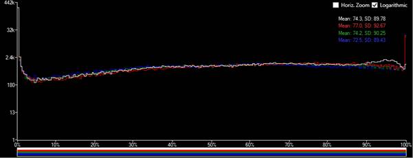
Clicking the FX Selection Area icon in the Tool Bar shows a red rectangle on the image which can be dragged and re-sized. While this selection area rectangle is enabled, the histogram is only calculated for the parts of the image within the rectangle.  This allows for more detailed scrutiny of a restricted region of the image and of how the histogram in the region appears.

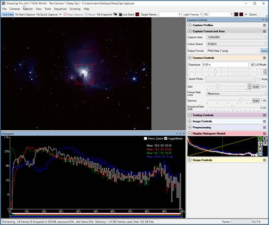
Notice the two histograms above are different but no camera settings have been changed.

The Histogram in Detail

Auto Hide – at the top right, the ‘pin’ icon can be used to auto hide the histogram when the mouse is moved away from it.  Moving the mouse back over the collapsed histogram tab will re-show it.

Horizontal Zoom selection – this checkbox can be used to zoom the horizontal axis by a factor of 3 to 5, allowing fine details in the histogram to be studied

Logarithmic/Linear selection – the checkbox will switch between a logarithmic vertical axis display and a linear display. Logarithmic tends to be a better way to see small values in the histogram that would otherwise be invisible due needing to show tall peaks elsewhere in the graph. When using the logarithmic option, remember to keep referring to the values shown on the vertical axis to see the number of pixels at each brightness level.

Mean and Standard Deviation (SD) – statistical information for each colour channel giving the mean and standard deviation of the pixel values for that channel. These are measured in ADU (Analogue to Digital Units) with a maximum value of 255 at 100% for 8-bit images and 65535 at 100% for 10/12/14/16-bit images.

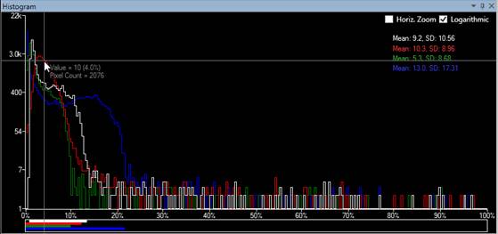
Crosshairs – these show when the mouse is moved over the histogram area and allow you to read off the ADU value and pixel count for any point on the histogram graph easily. Note that the readouts for both value (ADU level) and pixel count correspond to the horizontal and vertical positions of the crosshair. To read the number of pixels at a particular level, ensure that the crosshair is vertically at the level of the graph reading you wish to measure.        

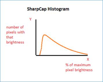
Horizontal axis – the % of maximum pixel brightness (in 8 bit modes the pixel brightness is 0 to 255, in 16 bit modes 0 to 65535).  This is scaled as 0 – 100 and caters for 8-bit, 12-bit, 14-bit and 16-bit cameras in a uniform presentation.

Vertical axis – the number of pixels at that brightness.

The Histogram Lines – The four lines on the histogram graph showing the brightness distribution of each of the three primary colour channels (Red, Green and Blue) and the distribution of the total brightness of each pixel (often referred to as Luminance).

Horizontal Colour Bars – these bars below the horizontal axis represent the ranges of the Luminance, Red, Green and Blue channels (commonly referred to as LRGB).

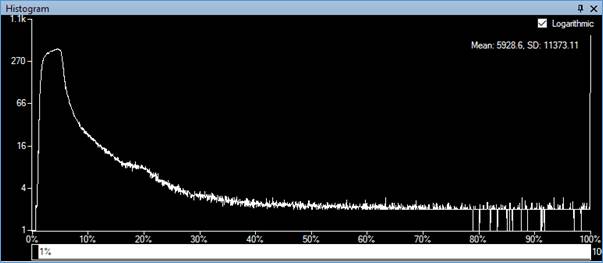
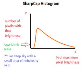
This histogram below conveys the following information:

· Approximately 400k pixels have 3% of maximum pixel brightness.  This is the histogram peak.

· Approximately 15 pixels have 100% of maximum pixel brightness”, that is, are saturated in this case.  This is a very small number of pixels compared to the total number in the image, so the clipping at the right-hand side is of little significance.

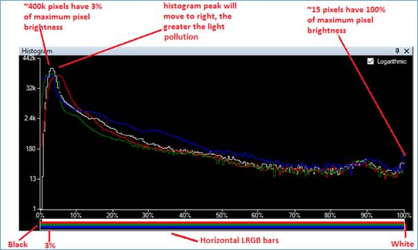
Note when using a Mono colour space, there is only a single white horizontal bar (Luminance) and single line on the graph.

Understanding the Histogram Axes

The diagram below defines the units of the horizontal and vertical axes. 

Note SharpCap shows the horizontal scale as a %, giving a uniform method of labelling to cover 8, 12, 14 and 16-bit cameras.

The horizontal scales can be found on the internet using a representation of the bit depth capability of the camera.  The table indicates alternate horizontal scales that may be encountered, the numbers being derived as 2ⁿ-1, where n = bit depth of camera.

Camera bit depth	Histogram horizontal scale
8	0..255
12	0..4095
14	0..16383
16	0..65535

Linear and Logarithmic Scales

By deselecting or selecting the Logarithmic checkbox at the top right, the shape of the SharpCap histogram can be changed.

Vertical scale is linear, checkbox not selected	Vertical scale is logarithmic, checkbox selected

In the graphics above, notice the vertical scales are different.  The following is a description of the difference between Linear and Logarithmic scales.

Note: ~ means approximately in the calculations.  The slight inaccuracies are due to rounding errors when scaling to fit the screen.

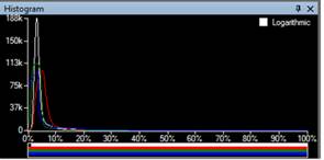
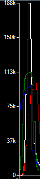
Linear Scale  is unchecked in the Image Histogram. · The numbers are uniform. · The tick marks are equally spaced. · The tick marks have uniform differences between their values. · The values are 0, 37k (1*37), 75k (~2*37), 113k (~3*37k), 150k (~4*37k), 188k (~5*37k). · The increment from one tick mark to the next is ~37k (37000), that is 37k is added to each value to get the next value. · If the graph is twice as high in one place (say at 50% brightness) as another (say 25% brightness), meaning there are twice as many pixels with 50% brightness as with 25% brightness.

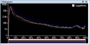
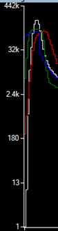
Logarithmic Scale  is checked in the Image Histogram. · The numbers are non-uniform. · The tick marks are equally spaced. · The tick marks do not have uniform differences when moving from one value to the next – instead they are multiplied by some amount.  For instance, the values are 13, 180 (~13*13), 2400 (~13*13*13) and so on.  · Those who can remember basic algebra, will recognise 13^0, 13^1, 13^2, 13^3 and so on. · The vertical scale increases the height of areas where there are small values and reduces the height where there are large values. · Becomes easier to see those parts of the graph with a much-reduced number of pixels at each level.  · Logarithmic scales help to get all the data on the chart so the values are readable – they supress the high values and enhance the low values.

After reading the above, the question is “Should a Logarithmic scale or a Linear scale be chosen when using the Image Histogram?”

The answer is “think about the type of object being imaged and use whichever obtains the best images” but, bear in mind the following:

· Linear makes most sense when the area the histogram is being applied to is roughly uniform in brightness, for instance:

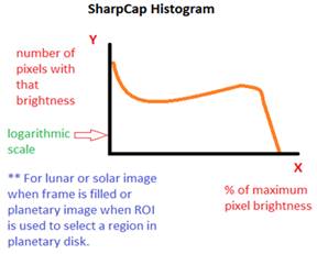
o A lunar or solar image when the frame is filled.

o A planetary image when the ROI is used to select a region inside the planetary disk.

· Logarithmic makes sense when there are distinct different regions inside the histogram area, for instance:

o A deep sky full frame containing a small area of nebulosity.

If the deep sky was looked at with a linear histogram, the peaks from the nebulosity and stars would be swamped by the vast black level peak and therefore invisible.  However, the logarithmic scale gets around this.

The following two examples both use a logarithmic scale but depending on the type of object being imaged (deep sky or large disk) the desired histogram shape is totally different.

Deep Sky	Large Disk

Using the Histogram to Improve Image Quality

The shape of a ‘good’ Histogram can vary depending on:

· A logarithmic or linear vertical scale being selected.

· The object being viewed:

o Deep Sky.

o Solar/Lunar/Planetary.

o Solar/Lunar/Planetary when ROI (Region of Interest) is used to select an area inside the disk.

Guidelines for ‘good’ histogram shapes for linear/logarithmic vertical scales and object types are summarised below.  Following these guidelines will help ensure images are correctly exposed.

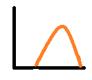
Deep sky - linear

Deep sky - logarithmic

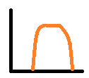
Solar/lunar/planetary – linear

Solar/lunar/planetary - logarithmic

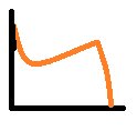
Solar/lunar/planetary with ROI or when target is filling frame (i.e. no black background) – linear

Solar/lunar/planetary with ROI - logarithmic

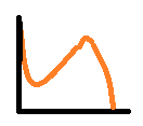
It is helpful to consider the following information to understand why these shapes of histogram are associated with the given types of image:

· Deep sky histograms have a peak at low intensity levels due to the dark background and typical low brightness of any nebulosity.

· Solar/lunar/planetary histograms usually have a peak near the black level due to the dark background and another peak for the (relatively) large and bright image of the target.

· Solar and Lunar histograms where an ROI is used or the sun/moon fill the entire frame will not have a peak near the black level as there is no black background.

The following two diagrams show the type of problems (plus suggested fixes) encountered with a histogram.

Under-exposed image

When the histogram looks like this (shifted too far left), the image is said to be under-exposed or black level clipped.  This will result in an image with a grainy background.  The grainy background is difficult to remove with post-processing software.  Faint detail will be hard to bring out.  To fix, expose the image for longer (preferred) and/or increase gain and/or increase brightness or offset.

Over-exposed image

When the histogram looks like this (shifted too far right), the image is said to be over-exposed.  Pixels in the image become saturated, resulting in detail being lost.  To fix, expose the image less (preferred) and/or reduce gain.

Quick Guides for Different Imaging Situations

Solar/Lunar/Planetary Imaging

Key goals:

· Short exposures to freeze seeing and allow for high frame rates

· No saturated pixels

· Reasonable image brightness of target

Method:

· Set an 8-bit mode (RAW8 or MONO8) to allow high frame rates.

· Consider using an ROI capture (smaller capture area) for planets to allow higher frame rate.

· Set a short exposure to allow a fast frame rate. For instance, 30ms will allow up to around 30fps.

· Reduce exposure further on brighter or fast changing targets (Sun, Moon, Jupiter) to get a higher frame rate. Once the frame rate stops increasing, the exposure is short enough.

· Increase gain to bring image brightness for the target up to a maximum level of about 85% on the histogram.

· If maximum gain reached, or image is excessively noisy, consider increasing exposure back up towards 30ms, meaning a reduced gain can be used.

· Use the Exposure/Gain Shift control to explore possible trade-offs between lower exposure/higher gain and longer exposure/lower gain. Longer exposures will reduce image noise but also reduce frame rate.

Note that H-alpha capture of the sun may benefit from high bit depths (MONO12-16) if you wish to try to capture both the photosphere and prominences at the same time. This will usually reduce the frame rate.

A correctly exposed histogram for planetary capture with a maximum brightness level of roughly 80% – the size of the peak on the left hand side will depend on the amount of dark sky surrounding the planet included in the measurement.

An under-exposed histogram for planetary capture – peak brightness levels reaching barely 50%, leaving the remainder of the camera’s range unused. Increase gain and/or exposure length to achieve correct exposure levels.

An over-exposed histogram for planetary capture – parts of the image are at 100% saturation, so image data is being lost. Reduce gain and/or exposure length to bring peak brightness levels below 90% saturation.

Note that when capturing a full frame surface (Solar, Lunar imaging), the left-hand side of the above histograms will not show the peak near 0% - instead falling away at the lowest brightness levels. The right-hand side will continue to show over/under/correct exposure in the same way.

Flat Frame Capture

Key goals:

· No saturated or nearly saturated pixels

· Minimize noise in final master flat

· Avoid low pixel values where noise will have large effect on flat correction calculations

Method:

· Use a high bit-depth mode (RAW12-16, MONO12-16) to capture maximum image detail

· Set low gain to minimize noise in frames (no need to take flats at same gain as lights)

· Adjust exposure while observing histogram.

· Avoid histogram reaching 100% or below 10% (if possible).

· Minimize histogram above 80% or below 30% (as much as possible).

Note that colour cameras and situations with strong vignetting or deep dust shadows may make it hard to obey all of the guidelines at the same time. It is however essential to avoid the histogram hitting 100%.

A reasonably well exposed histogram for flat capture. Ideally the peak green level would be lower than 90%, but this must be balanced against the weaker values of the blue channel not being too low.

An underexposed histogram for flat capture – all pixels in the blue channel are below 20% and the top half of the histogram range is completely unused.

An over-exposed histogram for flat capture. The green channel has pixels at the 100% level – in particular some pixels should really be higher than 100% and will not perform proper flat correction.

Deep Sky Imaging/EAA

Key goals:

· Capture at the highest available bit depth

· Avoid clipping the histogram on the left side for dark frames

· Set gain to reduce read noise (and hence reduce exposure length - if required)

· Exposure length must be long enough to minimize effects of read noise and keep number of frames captured to a reasonable level, but short enough not to risk bad frames due to poor tracking/guiding

Method:

· Set maximum bit depth (RAW12-16 or MONO12-16).

· Use Smart Histogram below to calculate the best gain and exposure times for your camera.

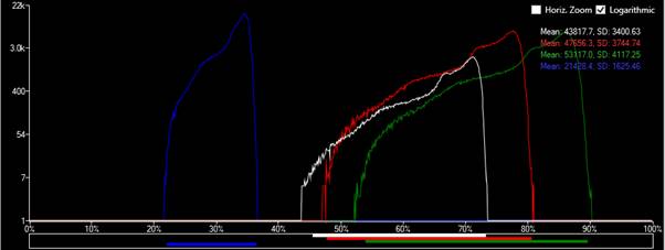
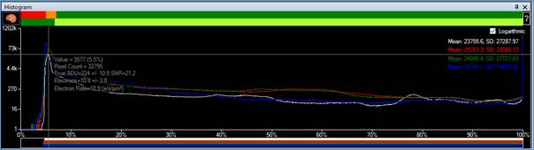
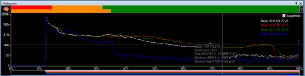
· Alternatively, examine the ‘Read noise vs Gain’ graph provided by your camera manufacturer – examples below

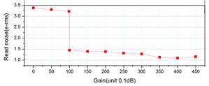
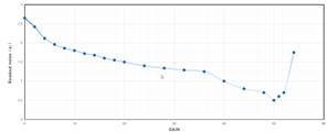
· Set a gain value just to the right of any big drop in the graph (i.e., gain 100 on the left-hand plot), or where the descending curve flattens somewhat (i.e., gain 20 to 30 on the right-hand plot).

· Cover the telescope and capture dark frames of 1s exposure. Adjust the Offset/Black Level/Brightness control to ensure that the peak in the histogram on the left-hand side does not touch the 0% level.

· Set a 30s exposure and take test images of the target.

· Increase exposure providing no poor star shapes from bad tracking/guiding and the only saturated areas of the image are bright stars.

· Decrease exposure/gain if you see trailing stars due to poor tracking or saturated areas of the image.

The exact procedure for setting exposure and gain for deep sky imaging is unfortunately complex, and a manual adjustment requires consideration of

1. Camera characteristics including how read noise varies with gain

2. Properties of any filters in use

3. The amount of light pollution in the area being imaged

4. The focal ratio of the telescope in use

5. The quality of tracking/guiding – how long can exposures be before glitching becomes obvious and frequent?

6. The total number and size on disk of saved images, along with the time taken to process them (shorter exposures will create more saved images over 1 hour of imaging).

The Smart Histogram calculation will take care of the points 1 to 4 above and allow you to limit the minimum and maximum exposure times that can be used to account for items 5 and 6.

A correctly set-up dark frame histogram for the adjustment of the Black Level/Offset/Brightness control. Note that the peak is effectively separated from the 0% level (maybe one or two pixels at 0% is fine). Note that the horizontal scale here only extends to about 20% due to the Horizontal Zoom function of the histogram being in use.

A histogram indicating that the Black Level/Offset/Brightness value needs to be increased due to some pixels having values at 0%.

Smart Histogram

Have you ever wondered whether you are using the right gain or exposure when deep sky imaging? Whether 6x ten-minute exposures really do give you more detail than 12x five-minute exposures? No more guesswork is required with the SharpCap Pro Smart Histogram feature. In combination with the results of Sensor Analysis, SharpCap can measure the sky background brightness for you and then perform a mathematical simulation of the impact on final stacked image quality of using different gain and exposure combinations. You can also see graphs showing the impact of using longer or shorter exposures (or lower or higher gain) than suggested.

If you try this using a modern, low noise, CMOS sensor you might be pleasantly surprised to find out that the optimal exposure length isn’t nearly as long as you imagine and that maybe the complexities of guiding will become a thing of the past (The use of long – 5 to 10 minute or even longer – exposures in traditional deep sky imaging is not required to see faint targets, it’s actually required to deal with the high typical read noise of CCD sensors. Since the optimal exposure length is proportional to the square of the read noise and CMOS read noises can be 1-3 electrons instead of 8-10 electrons, exposures can often be much shorter with no loss of quality).

Note that Smart Histogram functionality is only available for certain cameras:

· Smart Histogram is not available for any Cameras used via a DirectShow (Webcam) driver.

· Smart Histogram is only available for cameras that have been analysed using the Sensor Analysis tool. SharpCap ships with a selection of camera analysis data for the most popular Astronomy cameras, but you may need to run Sensor Analysis on each of your cameras to make the Smart Histogram features available.

The Smart Histogram Bars

The basic form of Smart Histogram takes the form of a pair of coloured bars along the top of the histogram area:

The top bar with the red, amber and green sections shows the impact of the camera’s read noise on the total image noise at that brightness level. For areas of the image in the red highlighted region of the histogram, the camera read noise dominates the total noise (more than 50% of total noise). In the amber region, the read noise contributes significantly to the total noise (10% to 50%). In the green region, the contribution from read noise is small (less than 10%).

The size of the red and orange zones will vary as you vary the gain and offset controls of your camera. Once you have picked values for those controls, you should adjust the exposure so that the histogram peak corresponding to the sky background is just to the right of the orange zone – this will give you optimum image quality without entering the zone where increased exposure time has diminishing (to zero) returns.

The lower bar indicates the effect of bit depth on the quality of captured image. In high bit depth modes (12, 14, 16 bit), the bar is green and light green (as seen above) – the light green section shows the range where the increased bit depth is not helping you because the total pixel noise equals or exceeds the distance between ADU levels in 8-bit mode. In the light green region, the use of high bit depth simply means that you are recording the pixel noise in greater detail!

In 8-bit modes, the lower bar is amber and green:

The amber region indicates the part of the histogram where you are throwing away data by using 8-bit mode (i.e. you would get more image quality by switching to 10/12/14/16 bits for parts of the image in this histogram region). The amber region will shrink to the left as you increase the camera gain level, and at the high gains used in planetary imaging it may not be visible at all – this shows why there is no need to use high bit depth modes for planetary ‘lucky’ imaging (and also that the Smart Histogram isn’t only useful for deep sky!).

The coloured bars at the top of the histogram are just the quick way to use the Smart Histogram features, giving you some basic guidance on exposure times and bit depths. For a more in-depth calculation that gives recommendations on gain, offset, exposure and bit depth, press the ‘Brain’ button next to the coloured bars to bring up the Brain window.

The Smart Histogram Brain Window

The ‘Brain’ window looks quite complicated, but if you follow it from top to bottom it should not be too hard to use.

The goal of the Brain is to help you pick the right camera settings to get the best deep sky images. Note that the Brain is not aiming to give you fabulous quality sub-exposure images, it is calculating how to get the best final image when you stack all frames taken in a set period of time (1 hour by default). The calculations will work out for you whether it is better to take 360 x 10 second images or 10 x 360 second images or some other combination. Note that the primary results (suggested exposure length and gain) do not change if you select longer or shorter total stacking times than the default value of 60 minutes.

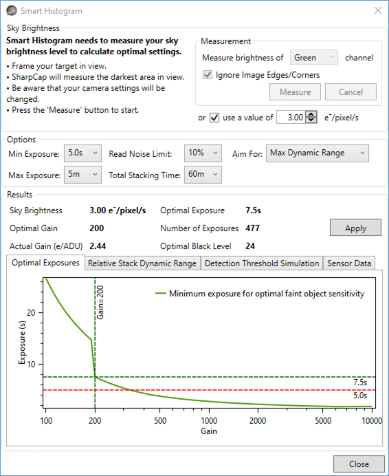
Measuring Sky Brightness

The first step is to measure (or enter) your sky brightness – this is measured in electrons per pixel per second and is a measure of how much signal is arriving at every pixel on your camera every second from sources that we don’t really want – light pollution and thermal noise being the main culprits. If you press the ‘Measure’ button then SharpCap will set the gain to maximum and take a number of increasing length exposures to measure this value – you should point the telescope at your target before taking a measurement – SharpCap will automatically measure the darkest region in the field of view of the camera.

For a colour camera, you may wish to choose which channel (red, green, blue or darkest) to measure. Often the blue channel will be the darkest and will therefore lead to longer exposures being recommended.

If you are using filters when imaging, you should measure the sky brightness with the filter in place – filters are often designed specifically to reduce the background sky brightness, and it is important for SharpCap to be able to take that effect into account. If you use multiple filters you may want to measure the sky brightness with each filter separately, or to work from the values given for the darkest filter.

If your imaging setup suffers from vignetting (darkening) near the edges/corners of the image, consider selecting the Ignore Image Edges/Corners option. This will stop SharpCap from taking those areas of the image into account in its measurement, making sure the calculations are optimised for the central area of the image.

Note that the sky brightness will vary depending on a number of factors such as the altitude of your target, sky transparency, proximity of a bright moon, etc.

After using the Brain Window a number of times, you may become familiar with typical values for sky brightness at your observing location and be able to enter the value directly by using the manual adjustment to specify an approximate sky brightness in e/pixel/s instead of performing a measurement.

Setting Limits and Targets

The next step is to set limits and targets for the calculation – you can set a minimum and maximum exposure to consider (typically maximum exposure is determined by mount tracking/guiding quality and minimum by how much data you have to save with very short frames or stacking speed for live stacking). You can also set the time you intend to image for (setting this value is not critical, changing this will *not* change the suggested values) and the contribution you are prepared to tolerate from the sensor read noise in the final image noise level. If you select a ‘Read Noise Limit’ of 10%, that means that the calculations will allow the total noise level in the final stacked image to increase by 10% above the minimum achievable noise level (i.e. to go from 10 to 11 on some arbitrary scale).

The last choice in this section determines how the gain is chosen – the two options are ‘Unity Gain’ which aims for 1 electron per ADU (or as close as possible) and ‘Max Dynamic Range’. ‘Max Dynamic Range’ finds the gain where the final stacked image will have the maximum ratio between the brightest thing that is not quite saturated and the noise level. Max Dynamic Range will often (but not always) choose the minimum gain value.

If ‘Max Dynamic Range’ is selected then the calculation takes account of the number of frames that can be captured (based on the exposure recommendation). If you choose ‘Max Dynamic Range’ and then use a longer exposure than the suggested one, you may be missing out on better alternative camera settings. It’s better to increase the Minimum Exposure setting in this case to force a longer exposure to be considered, which will result in a correct recommendation.

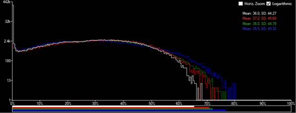
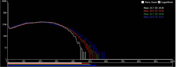
The Results

Once the sky background is measured and the limits and targets are set you can examine the results. In the image above, you can see that with a 5e/pixel/s sky brightness (quite bad light pollution), the calculation is recommending a gain value of 398, an exposure of 9.4s and a black level of zero (because the sky brightness will be enough to pull the histogram clear of the left-hand side). The graphs below show useful detail on the calculations that help you understand the result and if necessary tweak the values.

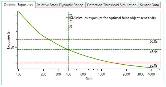
The optimal exposure chart shows you the exposure time you need to use to hit your ‘Read Noise Limit’ criteria for different gains – it also shows your minimum and maximum exposure limits as horizontal red lines if they fall within the range of the graph. From this graph we can see that in this case the recommended exposure is 46.9s at 398 gain, but an exposure of 60s could be used at 230 gain or 30s at about 1400 gain to get very similar results. You aim for at least the exposure time shown on this graph, although selecting a longer exposure won’t improve things much as we will see in the detection threshold simulation chart.

Note that the calculations performed here take into account only the visibility of faint detail above the noise level of the captured images. Other factors can also have an impact on the exposure/gain that you wish to use – for instance:

· You may wish to limit the number of frames captured or the size of the captured image files – this may prompt you to increase the exposure.

· You may wish to ensure that sufficient bright stars are shown in the image to allow stacking to work well – again this may prompt you to increase the exposure

· Light pollution might lead to a very high background level in longer exposures – this may prompt you to limit the exposure length

If any of these apply, causing you to want to adjust the recommended values, it’s a good idea to use the minimum/maximum sub-exposure times – for instance to specify a minimum exposure of 60s if you want to limit the number of frames captured. Doing this will ensure that you get the best recommendation for your situation – setting a minimum exposure of 60s may give different recommended gain and black level values to those give with a minimum exposure of 15s under some circumstances.

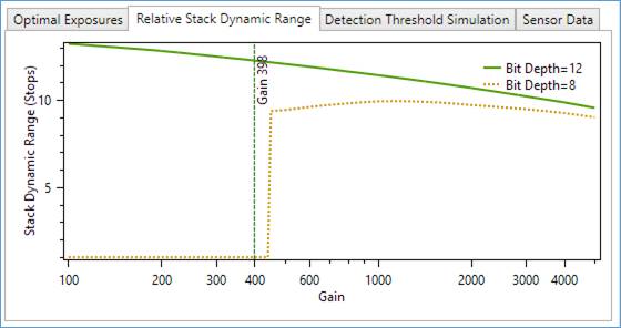
The relative stack dynamic range chart shows how the dynamic range of the final stacked image will be affected by changing the gain (assuming you follow the suggested exposure time for each gain value). This chart shows information for different bit depths if the required sensor analysis data is available. In this case the stack dynamic range for the 8-bit line drops to zero at gains below about 450. This happens when there are no valid solutions for the exposure time that fit all the limits you have chosen – for instance in this case a read noise limit of 10% would require exposures longer than the maximum exposure value of 5 minutes when in 8-bit mode with a gain less than 450. In this case (in common with many cameras), you can get a slight increase in the dynamic range of the final stacked image by moving to lower gain values.

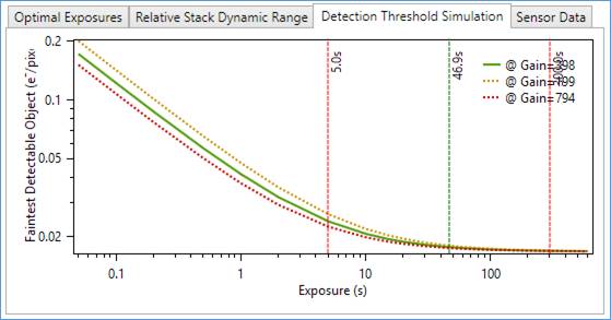
The third chart shows how the faintest visible object in the final stacked image varies with different exposure times. This chart makes it very clear how little extra final sensitivity you will achieve by exceeding the recommended exposure times. In this case at the recommended values (Gain=398, Exposure=47s), the expected faintest detectable object would be 0.0176 e/pixel/s. Increasing the exposure from ~47s to 300s drops that to 0.0168 e/pixel/s, an improvement of about 5%. You can also see that by this point the curves are basically flat – further increases in exposure bring practically no improvement to visibility of faint objects in the final stacked image.

You should use the figures recommended by the Smart Histogram feature as a starting point for fine-tuning the optimal settings for your imaging. For instance if you have good guiding and Smart Histogram recommends 30s exposures, you may wish to use somewhat longer exposures.

The Detection Threshold Simulation assumes that the faintest object you will be able to see in the final stacked image is equal in brightness to the noise level in that image. In fact, for objects that cover a large number of pixels, you might do a bit better than that as it is easier to see a large faint object than a small one, but this does not change the shape of the curve, in particular the fact that beyond the recommended exposure level there is practically no improvement in final image sensitivity to faint detail with further exposure increases.

In summary, when you use the Brain window, SharpCap simulates in a fraction of a second all the possible combinations of gain and exposure that you might use to image and calculates what the effect of each set of parameters would be on the final stacked image. This is possible because the results of the Sensor Analysis allow SharpCap to calculate the behaviour of the sensor for any combination of gain and exposure.

Smart Histogram requires a SharpCap Pro license and SharpCap needs sensor analysis data on each model of camera that you intend to use. SharpCap ships with sensor data for over 150 popular astronomy cameras, so you may find that Smart Histogram works for you straight away.

If you are using a camera that SharpCap does not have sensor data for, you must perform sensor analysis on each model of camera you intend to use. For best results perform sensor analysis in both 8-bit and high bit depth (12/14/16) modes.

Sensor Analysis

Camera manufacturers frequently produce charts of sensor gain, read noise and dynamic range for their cameras. Such charts are useful for comparing the characteristics of one sensor with another and also for helping choose the optimum camera settings for a particular imaging situation. However, until now, creating these charts was outside the reach of all but the most dedicated amateur astronomer, requiring as it did dozens of careful measurements and careful calculation.

SharpCap now automates the measurements and calculations required to perform this analysis on almost any camera (DirectShow cameras cannot be analysed because they do not have a fine-grained exposure control that SharpCap can adjust).

The results of the SharpCap Sensor Analysis procedure are used to support the Smart Histogram functionality that helps guide the choice of gain, exposure and bit depth when imaging.

Preparing to run a Sensor Analysis

These are the steps you need to carry out before running SharpCap’s Sensor Analysis tool.

· Ensure your camera is working well with SharpCap

· Set your camera into its highest bit depth mode, and if it is a colour camera, set it into RAW mode rather than RGB mode

· Find a source of constant illumination.

o Natural daylight on a clear or overcast day is ideal, but not on a day with scattered clouds as the brightness changes.

o Artificial light can work well but you may see lines in the image at short exposures due to the 50/60Hz flicker of many artificial lights – if this is the case then select a tall, thin area for measurement to include multiple flicker bands in the area

· Arrange for an evenly illuminated area to show in the camera field of view. Note that the whole field of view does not need to be evenly illuminated, just an area of at least 100x100 pixels. You can do this by

o Using your telescope, putting it out of focus and pointing it at the cloudy or blue sky or putting a white T-shirt or similar over the lens.

o Using a translucent 1.25” dust cap over the nosepiece of the camera

o Using a CS or C thread lens and pointing the camera at an evenly illuminated featureless object (like a sheet of paper)

o Using the camera with no lens or cover (but beware getting dust on the sensor).

· Arrange to be able to vary the brightness of the illumination of the sensor. You may need to do this to get the process to run to completion successfully (note: avoid changing the illumination brightness during the run – you may need to adjust at the beginning to get the right brightness to start).

· Arrange to be able to cover the sensor so that dark measurements can be made

· Set any colour balance, gamma or contrast controls for the camera to their ‘Neutral’ state.

· If your camera has a physical shutter (DSLR) or takes a long time to download a frame (large CCD), put the camera into Still Mode.

Running Sensor Analysis

To begin the process, select Sensor Analysis from the Tools menu. Any existing tool (such as the Histogram or Live Stacking) will close and the Sensor Analysis will open. The selection area rectangle will also appear in the image preview area.

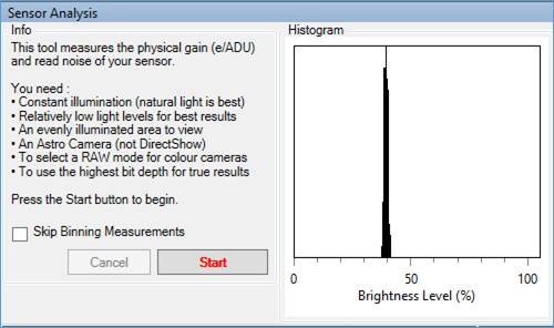
Some basic instructions and a small image histogram will show in the Sensor Analysis tool window. Only check the Skip Binning Measurements checkbox if sensor analysis has failed or become stuck at the final stage of measuring the effects of binning in a previous run. Once you have checked you are ready, press the Start button.

Selecting the Measurement Area

Once the Start button is pressed, SharpCap will automatically select the lowest gain level of your camera. SharpCap will also automatically adjust the camera exposure to correctly expose the region inside the Selection Rectangle.

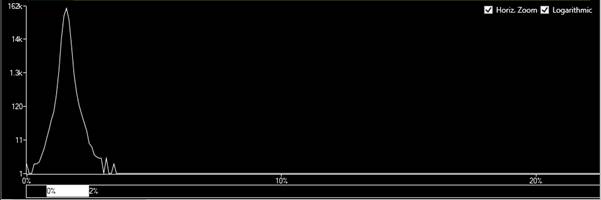
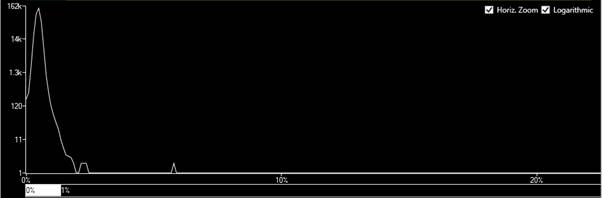
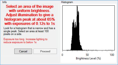
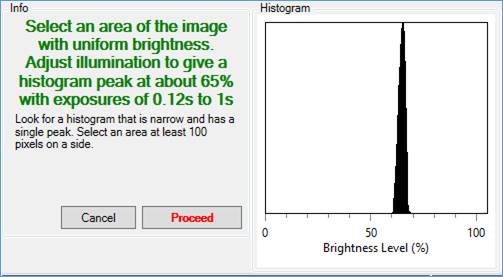
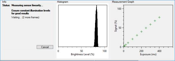
At this point you should adjust the move and/or resize the Selection Rectangle to select a region of the image that is of uniform brightness and colour. A suitable area of image will show a histogram similar to the one below with a single, symmetric peak towards the right-hand side. You should also adjust the brightness of illumination to give an exposure time in the range suggested. SharpCap calculates the required range based on the characteristics of your camera to try to ensure that the whole analysis procedure can be carried out with exposures under 2s and well above the camera’s minimum exposure.

Do not adjust the exposure value yourself – it will be automatically adjusted as you change the illumination levels or adjust the selection area.

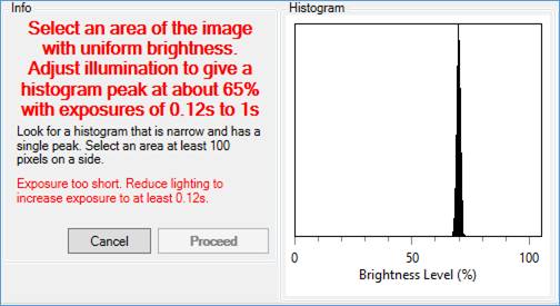
If the selected area is not uniform then the histogram will have more than one peak or an asymmetric peak. If the exposure time is too long or too short then a warning message will be shown in red giving instructions on what changes need to be made. Both of these situations are shown in the image below.

Once the light levels have been adjusted correctly and the selection area chosen, press the Proceed button to start the actual measurements.

During the measurement period, be careful not to

· Disturb the camera while measurements are being taken

· Move in front of the camera (which will change the light levels being measured)

· Allow the light level reaching the camera to change (except when asked to cover/uncover the sensor).

· Adjust any of the camera controls manually – making manual adjustments will very likely cause inaccurate or invalid results.

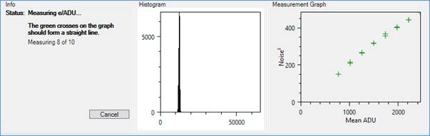
Bit Depth and e/ADU Measurements

The first stages of sensor measurement involve measuring the true bit depth of the images that the camera produces and the e/ADU (electrons per ADU) of the camera at minimum gain. While the e/ADU measurements are being made a scatter graph will draw to the right of the histogram which shows the relationship between measured frame noise and measured mean ADU at various exposures. The green crosses should be close to a straight line.

After this stage is complete, the sensor must be covered so that no light can reach it to allow dark measurements to be made.

Linearity and Gain Range Measurements

The next stage measures the linearity of the sensor response to changing exposure time and also makes a rough measurement of the effect of the camera’s gain control. It’s particularly important not to allow the light level to change during these measurements – the most likely cause of a low sensor linearity limit in the final results is a variation of light level during measurement.

Dark Measurements

SharpCap will prompt you to cover the sensor to allow dark measurements to proceed.

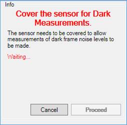
SharpCap will set a high gain and a 100ms exposure which will most likely lead to a white image showing on screen at this point. When you cover the sensor, the camera image will go dark and the Proceed button will become enabled. Press the Proceed button when it becomes enabled and the sensor is fully covered.

A large number of dark measurements need to be made, but they typically proceed fairly quickly unless the frame rate is very low. The initial measurements are of the brightness of the image with different values set for the Gain and Offset controls (Offset is also known as Black Level or Brightness). These are followed by measurements of the amount of noise present in dark frames at various gain values.

When the dark measurements are complete, the sensor must be uncovered to allow the final Gain and Binning measurements to take place.

Gain and Binning Measurements

SharpCap will prompt you to uncover the sensor.

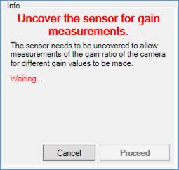
Once you uncover the sensor, SharpCap will begin to adjust the exposure to correctly exposure the selection area. At this point, you may (if required) adjust the brightness of illumination and the selection area as you did initially to ensure the area being measured is uniform and the exposure is in the recommended range. Once any necessary adjustments have been made, press the Proceed button, which will become enabled when the sensor is uncovered. Do not make any further adjustments after the Proceed button is pressed.

After you press the Proceed button, the final stages of sensor measurements will commence, which involve gradually adjusting the camera gain and measuring how much the exposure must be changed to counteract each change in gain. It is vitally important that the brightness of illumination of the camera does not alter during this part of the measurement process, otherwise incorrect results will be produced.

The final step is to briefly adjust the Binning setting of the camera to determine how the camera deals with binning, after which the results will be shown.

Sensor Analysis Results

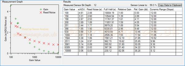
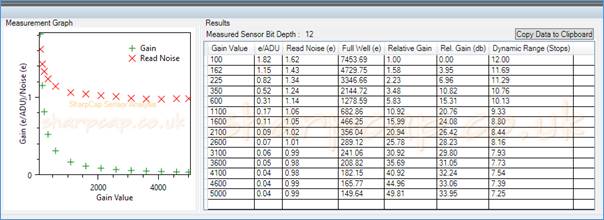
The primary results of the measurement process are

· The sensor bit depth, shown above the results table, here 12 bits meaning that the sensor can produce 2¹² (4096) different ADU values (different brightness levels).

· The e/ADU values for different gain settings, shown as the green crosses on the graph and in the table. This figure is the number of electrons required per pixel to increase the brightness measured by the camera by 1 ADU

· The Read noise of the camera for different gain settings, shown as the red crosses on the graph and in the results table. This is the amount of noise (in electron equivalents) that is added to each image due to the camera electronics not being perfect at reading the brightness of each pixel.

The other results, shown in the table are

· The Full Well capacity of a pixel – that is the number of electrons that it can hold before it becomes saturated (gives a 100% white signal).

· The Relative Gain for each gain setting, measured as a multiplier of the minimum gain or in dB

· The Dynamic Range for each gain setting – this is the ratio between the brightest signal that can be properly measured (the full well signal) and the dimmest (the read noise). This value is measured in photographic stops (effectively powers of two).

Usually, the graphs will show two smooth curves, with the highest values for both e/ADU gain and read noise at the left-hand side. The example above shows a sharp drop in the read noise at a gain value of approximately 200. In this case, the camera sensor switches to a more sensitive and lower noise mode when the gain is higher than 200 and this is reflected in the measurements.

SharpCap stores the results of completed Sensor Analyses on your computer and will use them later to provide Smart Histogram functionality on analysed cameras. If you re-run the analysis then the previous saved version will be overwritten. Note that previously saved sensor data will not be shown when you re-select the Sensor Analysis tool. It can however be viewed in one of the tabs of The Smart Histogram Brain Window.

To gain full Smart Histogram functionality, you should analyse your camera at both its maximum bit depth (i.e. in RAW12/RAW16/MONO16 mode) and at a bit depth of 8 bits (i.e. in RAW8/MONO8 mode).

Sensor analysis is a free feature and does not require a SharpCap Pro license, however users with a SharpCap Pro license can copy the table of values from the results if they wish.

Note: Sensor Analysis can be run with the camera in Still Mode. This is recommended for cameras with a physical shutter (such as DSLR cameras) and for high resolution CCD cameras that take a long time to download frames.

Sensor Analysis Data Files

Sensor Analysis data is stored in files saved in the folder

%APPDATA%\SharpCap\SensorCharacteristics

alternatively, you can access this folder as

C:\Users\<your windows user name>\AppData\Roaming\SharpCap\SensorCharacteristics

You can copy sensor analysis files from one computer to the same folder location on another computer to avoid having to run the analysis on each computer.

If you have a SharpCap Pro license then these files can be opened in a text editor and you can inspect the data that they store. If you do not have a SharpCap Pro license then these files are encrypted so that only SharpCap can read them (copying the data from the analysis results or access the data via the data file is a SharpCap Pro feature).

Focusing

SharpCap has a several options to help acquire focus on targets (possibly one of the most challenging aspects of astrophotography).  The tools are particularly powerful if an ASCOM focuser is configured in SharpCap (An ASCOM focuser is a device which uses a stepper motor or DC motor to move the telescope focuser and can be controlled from a computer via a USB cable).

Introduction

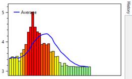
There are six Focus Score tools, the appropriate one must be chosen for the target.  Each tool attempts to measure the quality of focus of the image (the different tools measure the quality of focus by different methods) and displays the measurement in the work area as both figures and a graph.  The graph may look something like this:

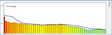
Green bars always indicate better focus while red bars always indicate poorer focus. The most recent measurements are shown at the right-hand side of the graph with older measurements to the left. Note, for some tools the best focus is associated with low scores (short bars in the graph), while for others it is associated with high scores (tall bars in the graph) – the best scores will always be green though.

It is possible to just select one of the focus tools and adjust the focuser until obtaining the best score such that the score can no longer be improved by moving the focuser in either direction, but better results can be obtained with a methodical approach and an understanding of how the process works and the adjustments available.

Don't try to use the focus tools if the image is a long way out of focus.  The tools are to be used to go from being close to focus to perfectly in focus.  If focus is a long way out and there are problems getting anywhere near focus, try one of the following:

· Focus on a terrestrial object at least 200m away in daylight (the further the better), which will get close to the focus point for astronomical objects.

· Use the moon, if it is visible, as it is easy to find and bright.  This helps because it can be hard to find any objects when the telescope is a long way out of focus.  However, the moon is bright enough to be hard to miss even when the focus is very bad.

• With high gain and exposure of 2s or so, aim at a bright star or planet.  Increase the brightness of the displayed image by one of the following:
• • Reducing the mid-level value for the display stretch or using display auto stretch.
  • Selecting 'Image Boost' from the FX dropdown.
  • Selecting 'Image Boost More' from the FX dropdown.

If the bright object is either in or near the field of view, all or part of a bright donut (reflector/SCT) or bright disk (refractor) of light will be seen – this is the very out-of-focus view of the object, made visible by the high gain and brightness boost.  Adjust the focuser of the telescope to make the disk/donut smaller, which will bring the telescope nearer to correct focus.

Understanding the Focusing Display

When selecting one of theFocus Score tools, Contrast (Edge) Detection in this case, the following screen appears.  This screen layout is the same for all six Focus Score tools.

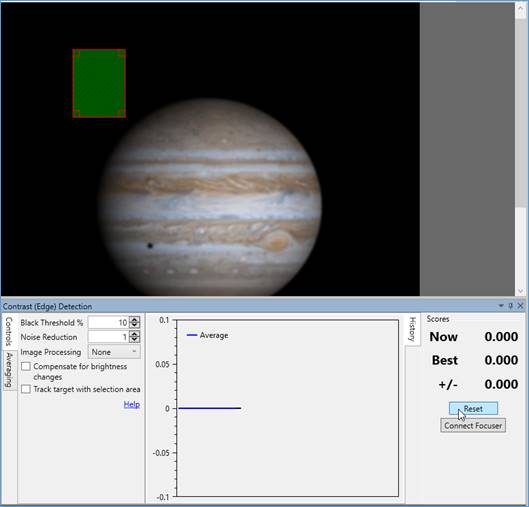
There are four distinct regions when a Contrast Focus Score tool is in use.

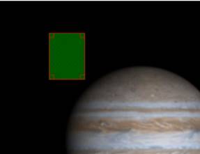
The Capture Display Area

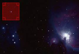
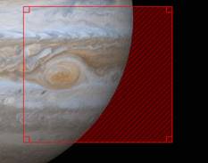
In the Capture Display Area, a red Selection Area rectangle appears.  The rectangle can be dragged with the mouse and resized.  It should be moved over the edge of the object, completely onto the surface, or expanded to surround the complete object.  · Any area outside the red rectangle will be excluded from focus score calculations. · Any area within the rectangle which is not shaded (above the black level) will be included for focus score calculations. · Any area within the rectangle which is shaded will be excluded from focus score calculations. These areas are below the Black Level and considered to be part of the background. Adjust the Black Level on the left if the wrong areas are being shaded.

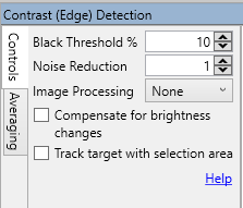
The Controls Pane

· Various controls may be available depending on which focus score has been selected. See the focusing tools  and Focus Tool Settings sections for more detail. · Brief Help for each tool is available.

The Graphs Pane

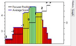
	· The graph region will display a plot for: Focus Score history (History tab) · The black line is used to indicate Focuser Position (only shown if a focuser is connected, explained later). · The blue line is Average Score – an average of the 10 previous focus scores. · The left hand vertical axis shows focus scores. · The right hand vertical axis shows focuser position.
	· Alternatively, you can show the Focus Score v Focus Position graph (Graph tab).  [Note: This only shows if there is an ASCOM focuser connected.] · The triangles represent focus measurements and different focuser positions – green when moving in the positive direction and red for negative movements

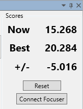
The Scores Pane

· The title bar of the panel can be used to drag the panel out of the main SharpCap window, for example to place it on a second monitor · The Pin icon can autohide the focus tool displayed in the Work Area. · Current score (Now) and Best score recorded so far (Best) are shown. · The Reset button clears the history and the best score.  If the Selection Area is enabled, disabled or moved, or the Black Level changed, the Reset button should be used. · If an ASCOM focuser is configured, but not connected, the Connect Focuser button will appear as an easy way to connect to your focuser and enable advanced features in the focus tools.

The Graph Pane

The History tab always appears (1st diagram below).  The additional Graph tab will only appear when an ASCOM focuser is connected (2nd diagram below). 

History Tab

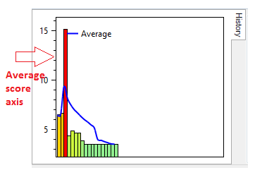
The History tab shows the history of focus score values in a column graph with the oldest measurements on the left and the most recent measurements being added on the right.

The History tab is the default tab when you do not have an ASCOM focuser connected. While it can be used with an ASCOM focuser, the Graph tab is better suited for use with focusers.

No ASCOM focuser connected

· Blue 'average' line appears, an average of the last 10 focus score measurements, helps to see changes when the focus value is varying from frame to frame due to noise. · New measurements appear on the right, older ones will disappear from the left once the chart area is filled.

ASCOM focuser connected

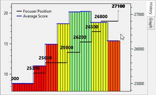
· Focuser Position axis on the right appears. · Black Focuser Position line appears. · Blue average line changes to a stepped graph. · Each horizontal segment of the average line corresponds to a period when the ASCOM focuser was at a certain position. · When the focuser position moves, a new segment starts. · The horizontal segments indicate the average focus score value over all the samples when the focuser was at that certain position.

This is the range of colours that can be displayed – from red (poor focus) to green (good focus).

Red > Orange > Yellow > Light Green > Dark Green

Colours and heights of focus graph bars are not an absolute measure of 'good focus', they are a measure relative to the other recent focus measurements made.  The best focus score recently obtained will always get a vivid green bar and will be the highest (lowest for FWHM) one in the graph.  This doesn't mean perfect focus; it means the best focus achieved since the focus tool was opened (or since last reset).  The exception to this is the Bahtinov mask tool - there the value of zero is an absolute measure of perfect focus.

Graph Tab

This graph only appears if an ASCOM focuser has been configured in SharpCap and is connected. In that case it becomes the default tab (although you can switch back to the History tab if you wish).

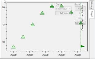
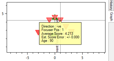
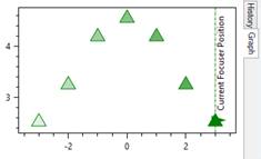
The Graph tab shows how the focus score measurements have varied with focuser position, with the focuser position being measured along the horizontal axis and the focus score being measured on the vertical axis.

Best focus is indicated by either a peak (maximum) at one point on the graph (contrast based focus scores) or a trough (minimum) at one point (star based focus scores).

The graphic shows the focuser position was stepped from -3 to +3 in the following sequence:

-3   -2   -1   0   1   2   3

This graph shows the focuser position along the horizontal axis and the focus score on the vertical axis.

· The green upward pointing triangles show data points collected when the focuser was moving in the positive (outward) direction.

· The red downward pointing triangles show data points collected while the focuser was moving in the negative (inward) direction.

· Stronger colours indicate more recent data points.

· Faded colours indicate older data points.

The black lines and numbers on the History graph below correspond to the focuser positions shown in the Graph above.

With an ASCOM focuser installed, work from the Graph tab rather than the Histogram tab.  To find the point of best focus using the focus score axis (at the left of the graph) look for:

· The peak value (Contrast Detection/Fourier options).

· Minimum value (FWHM options).

· Zero (Bahtinov option).

Note: This functionality can be experimented with using the Focus Offset control available in two Test Cameras. The focus offset control can be found in the Camera Control Panel, and will apply blurring to any image when it is set to a non-zero value. This control is only available if an ASCOM Focuser is not configured in the SharpCap settings (i.e. set the choice of ASCOM focuser to None to use this feature).

History and Graph Manipulation

· Drag with left mouse button to move around.

· Mouse wheel to zoom.

· Select an area with middle or right mouse button to zoom to that area.

· Double click to return to default view if lost.

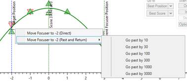
· Right click on the Graph area to show options for moving the ASCOM focuser to the position where you right-clicked.

	Hovering the mouse over the blue line will show focus score history of the preceding 10 samples.
	Hovering the mouse over the focuser graphics will display a focuser position and score report.
	Right-clicking on the graph allows you to command the focuser to move to the position that you clicked on. Movement can either be direct or a ‘move past and return’ movement which can help deal with focuser backlash.

Focus Tool Settings

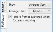
Each focus tool has settings for averaging – these setting control how many focus readings are averaged before adding a data point to the graph.

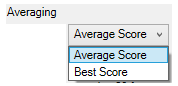
	Averaging – choose either average or best score from an averaging period to be the value recorded.
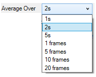
	Average Over – the period can be specified as either number of frames or a time-period by the settings offered. Averaging is more useful for high speed imaging (lunar/solar/planetary) – for deep sky imaging, setting the Average Over option to 1 frame is usually sufficient.
	Ignore frames captured when focuser is moving – this option is available when SharpCap is configured to use an ASCOM focuser. When enabled, SharpCap will ignore the focus score from any frame where the time over which the frame was captured overlaps with any time during which the focuser was moving. This is best left enabled to exclude possibly blurred frames from analysis

The tools also have settings to control the focus detection calculations – these vary from tool to tool. Most tools have some of the following options:

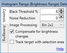
	Black threshold – anything below that level is excluded from the calculation, avoids including dark level noise in the calculation. The level is measured in terms of the percentage of maximum brightness.
	Noise Reduction – applies a Gaussian blur to the image to cut down on pixel noise before performing the measurement. The amount of blurring can be adjusted. Note that the blurring is not shown in the image on screen when this is adjusted.
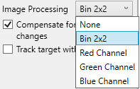
	Image Processing – available for all focus tools except for FWHM measurement tools. This allows you to apply simple image processing to the image before the focus measurement is calculated. Options are: · None – no image processing · Bin 2x2 – apply 2 by 2 binning, which will create a monochrome image for colour cameras · Select one of the colour channels (for colour cameras only). Selecting binning or one of the colour channels can help prevent the focus algorithm from picking up spurious detail from the bayer pattern in the raw image. The colour channel options can be used to focus specifically for one colour (in the case where the telescope may show chromatic aberration).
	Compensate for brightness changes – when enabled, SharpCap will attempt to calculate focus scores that are unaffected (or less affected) by the target changing brightness slightly. This can help if there are variable amounts of thin clouds when lunar, planetary or solar imaging
	Track target with selection area – This option is designed to help achieve good measurements when focusing on planetary targets (or solar/lunar if the whole disk is in view). If this option is selected and the Selection Area feature is enabled, SharpCap will monitor the position of the brightest object in the image and try to keep the selection area in a constant position relative to that object. This should allow the same are of a planetary or lunar/solar disk to be measured even if the target is drifting or is not steady.

Each focus tool also has a small amount of built-in help available that can be shown by clicking or hovering over the ‘Help’ link.  For example, this is the Help for Contrast (Edge) Detection:

The Focusing Tools in Detail

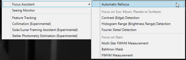
The six available focusing tools can all be found under the Calculate Focus Score icon from the Tool Bar.  Select the desired tool to begin measuring focus. The tools come in two groups – one that is suitable for focusing on the Sun, Moon, Planets or a surface, the other group is suitable for focusing on stars.

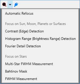
Contrast (Edge) Detection

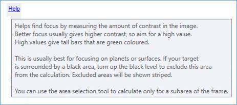
Suitable for planetary or surface targets.  Measures the total amount of contrast in the image - better focus gives more contrast which gives higher scores.

Tall green bars (high values) indicate the most contrast and hence best focus. Short red bars (lowest values) indicate the worst focus.

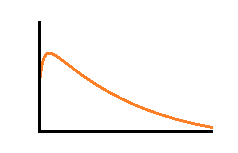
Histogram Range (Brightness Range) Detection

Suitable for planetary or surface targets (especially high noise).  Measures the range between the brightest and dimmest parts of the image - better focus should give higher scores. May work better for noisy (high gain) images than Contrast (Edge) Detection.

Tall green bars (high values) indicate the most contrast and hence best focus. Short red bars (lowest values) indicate the worst focus.

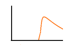
Fourier Detail Detection

Suitable for planetary or surface targets.  Measures focus by examining amount of detail in small scales in the image as determined by a Fourier Transform.  Good focus leads to higher scores.  May be less sensitive to noise than contrast detection options.

Tall green bars (high values) indicate the most contrast and hence best focus. Short red bars (lowest values) indicate the worst focus.

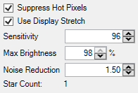
Multi-Star FWHM Measurement

Suitable for stars and point sources.  Measures the FWHM (Full-width, Half Maximum – a measure of the width of the star) of all suitable stars in the frame, giving an average score.  When a frame is out of focus, stars appear larger, making this measurement increase, so smaller values mean better focus.

The Multi-Star FWHM score has a number of controls to adjust star detection. You should adjust these controls to try to detect at least 20 stars (but no more than a few hundred). Guidance on adjusting these controls can be found below.

At least five suitable stars must be detected for a valid score to be generated – if less than five stars are detected then a placeholder score of 25 is reported.

Note that SharpCap actually calculates an estimate of the Half Flux Diameter (HFD), which is a measure closely related to the FWHM. The HFD is, however, less affected by noise in the image than a direct measurement of the FWHM.

	Suppress Hot Pixels – Enabling this option adjusts the star detection process to avoid detecting a star from a single hot pixel in the image. You may need to turn this off if you are using a large pixel camera and a short focal length telescope (i.e. your stars are very small).
	Use Display Stretch – when this option is selected, any display stretch applied to the image is also used for star detection to help detect faint stars. In general, leave this option selected.
	Sensitivity – This controls the overall sensitivity of the star detection process – increase this value to try to detect more stars, decrease it to reduce the number of stars being detected. Note the following: · Setting a higher sensitivity can make star detection take longer, potentially slowing down the stacking process · SharpCap will auto-adjust the sensitivity for you, turning it down (to a minimum of 75) if more than 200 stars are detected and turning it up (to a maximum of 75) if less than 25 stars are detected.
	Max Brightness – this is the maximum brightness level for stars to be considered for part of the FWHM measurement. Fully saturated stars are not included as it is impossible to tell how over-saturated they are, meaning that they can give inaccurate results.
	Noise Reduction – when enabled applies a Gaussian blur to help SharpCap to ignore low level noise and hot pixels.  Increasing this may help detect stars correctly in noisy images.

Short green bars (low values) are indicated best focus.  Red bars (highest values) indicate worst focus.

Note that this option actually measures the half-flux-diameter, a property that is closely related to the FWHM, but is not so badly affected by noise or mis-shaped stars.

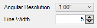
Bahtinov Mask

Suitable for stars or other point sources.  Requires a Bahtinov mask to be placed over the aperture of the scope and the area around the star and lines to be selected using the selection tool.  Best focus is achieved when all three lines intersect at the same point which gives scores (positive or negative) closest to zero.

A Bahtinov mask of suitable diameter must be placed over the end of the telescope to use the Bahtinov Focus Score tool.  Negative values are possible, values nearest zero are best, so -0.1 and 0.1 are equally good, 0.0 is perfect and +3.9 and -3.9 are equally bad.

Angular Resolution and Line Width are controls found only in the Bahtinov focus score.

Angular Resolution – measured in degrees and defines how finely to scan the full 360 degrees when looking for Bahtinov lines – the default scans once per degree, but it can be made finer.  Possible values are 0.20°, 0.25°, 0.33°, 0.5°, 1.0° Line width – measured in pixels and should be set to roughly the width of the Bahtinov spikes seen on the screen – the correct value here helps SharpCap separate the spikes from the noise.  Possible values are 1..40 in increments of 5.

Short green bars (low values) are best – values can be positive, negative or zero.  A value of zero indicates best focus.  Red bars with large values (either positive or negative) are worst.

FWHM Measurement

Suitable for stars or other point sources.  Measures the width (FWHM) of a single star –  which must be selected using the selection area tool.  Better focus gives narrower stars and a lower FWHM score.

Multi-Star FWHM is usually better than single-star because it takes 10s or 100s of FWHM measurements and averages them, so there should be less noise and less systematic error in the reading.

Short green bars (low values) are indicated best focus.  Red bars (highest values) indicate worst focus.

Which Focus Tool Should Be Used?

For a field of view with many visible stars, use Multi-Star FWHM.

For a single-star (or sparse) field use either FWHM or Bahtinov Mask.

For planetary or surface targets, there are three tools to choose from:

· Contrast (Edge) Detection

· Contrast (Brightness Range) Detection

· Fourier Detail Detection

When trying to focus a planetary or surface target consider the following:

· The different focus score algorithms are attempts to find a better balance between two opposing factors – sensitivity to being in good focus and insensitivity to noise.

· There are trade-offs involved in the various approaches.  Which to use is going to be a matter of trial and error and/or personal preference.  The Contrast (Edge) Detection tool is (probably) a good starting point in most circumstances.

Focusing Procedure

The table details the various steps to be followed to achieve good focus of the telescope.

Telescope (no ASCOM focuser)	Telescope (with ASCOM focuser)
Preparation Phase · Initial visual focus with camera and telescope against a distant object.
Setup Phase · Check target not over exposed using Image Histogram tool. · Select appropriate Calculate Focus Score tool – adjust black level, target detection parameters, ROI box – to obtain best focus score. · Reset the graph to wipe the score history.
Focusing Phase · Adjust telescope focuser manually, watch focus scores.  Stop when best score obtained. · Telescope now in focus.	Focusing Phase · Adjust telescope focuser using the Focuser controls in the camera control panel, watch focus scores · Use the Graph tab.  Stop when best score obtained. · Telescope now in focus.

During the Setup Phase, the scores being shown are meaningless as they are changing because of changing the software parameters, not changing the focus of the telescope.

At the end of the Setup Phase, Reset the Graph to wipe the score history.

During the Focusing Phase, only adjust the telescope's focuser, not any of the settings within SharpCap – this is to ensure the changes seen in the focus score are only a result of the changes in focus of the telescope and are not influenced by anything else.  If any SharpCap settings are changed during the focusing stage (for instance because a planetary target has shifted in the field of view and there is a need to update the ROI), reset the graph after making the adjustment – effectively starting the focusing phase again.

Focus will need to be checked throughout a session as it could change because of one or more of the following factors:

· Change in temperature affecting telescope tube.

· Change in temperature affecting optics.

· Changing filter

· Mechanical slippage (creep) of the focuser under heavy camera loading

The table below shows what would be seen in SharpCap when using the appropriate Calculate Focus Score tool for a telescope both without and with an ASCOM focuser.

Telescope (no ASCOM focuser)	Telescope (with ASCOM focuser)
FWHM measurement for star. In this trace, the focuser was moved from a position of reasonable focus (initial yellow/green bars) to a position of poor focus (red bars) and back to a position of good focus (dark green bars).  [Note: History tab only.]	Contrast Edge Detection for a planet. In this case, the focuser was moved from an initial poor focus to a better focus and past best focus back to a poor focus position.  [Note: History and Graph tabs.]

(Nearly) Automatic Focusing

When using an ASCOM focuser, SharpCap Pro users can activate additional features that allow many of the steps outlined above to be automated. The actions that can be automated are

· Scanning over a range of focuser positions, measuring the focus score at each position to produce a focus quality graph automatically.

· Returning automatically to the position at which the best focus score was measured

· Refocusing completely automatically re-using the settings from the last successful focus scan

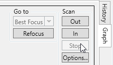
All of these functions can be activated using the controls which are available in the top-right corner of the Focus Graph

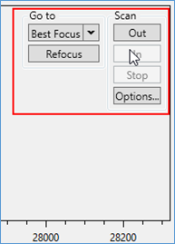
Note that the buttons in the Goto and Scan groups will appear slightly transparent until you move your mouse over them – this allows graph detail behind the buttons to be seen.

Automatic Focus Scanning

The Scan In and Scan Out buttons can be used to initiate an automatic scan over a range of focuser positions, measuring the quality of focus at each position. This is best started one side of the point of best focus so that the scan will pass through the expected position of best focus.

The scan will continue, building up data in the Focus Graph until either

· The Stop button is pressed

· The focuser reaches its maximum or minimum possible position

· The number of steps configured in the options has been completed

· A best focus position has been found (if Smart Scanning is enabled).

During the scanning process, information on progress will be shown in the notification bar.

Point of Best Focus Detection

SharpCap will monitor the focus data being accumulated during both automatic and manual focus movements and try to find a pattern in the data. In particular SharpCap is looking for the point of best focus, which will be indicated by a best-fit curve with either a peak (as shown below) or a valley. A valley shaped best-fit curve should be expected for focus scores where the lowest values are best (i.e. star FWHM measurements), a peak should be expected for scores where the highest values are best (i.e. contrast measurements).

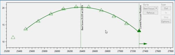
The best-fit curve will indicate the position where best focus is expected to be found, even if it occurs between two measurement positions.

Note that the focus measurements must include at least three measurements each side of the point of best focus for the focus best-fit curve to be detected properly. If a focus scan stops at or before this point (i.e. the stopping point has the best score so far) then press the scan button again to continue the scan past the point of best focus.

A best fit curve will only show if there is a relatively strong pattern in the measurements showing a peak or a dip in the focus score. If the focus measurements are very variable with no distinct pattern then a curve will not appear. This problem is often caused by the movement of the focuser being within the ‘backlash’ region, such that even though the motor is turning the focuser itself is not moving the camera.

Once the best-fit curve is shown and has a clear peak or valley, the Go To Best Focus button can be used to return the focuser to the point where the best focus was achieved.

Returning to Best Focus

SharpCap can return to either the focuser position where the best focus score was obtained using the Go To Best Focus button.

This button has a dropdown to allow choice of which direction of movement to use the best data from – positive (outward) or negative (inward). The Focus Graph can show two best fit lines (green for movement in the outward direction, red for movement in the inward direction). If the focuser hardware has any significant backlash then these lines may not peak in the same position, making it important to be able to choose between them.

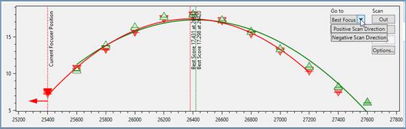
The default action of the Go To button (if you do not choose from the dropdown but just press the button) is to choose the direction that was scanned most recently. When this button is pressed, SharpCap will calculate the focuser position for the optimum point on the best-fit curve and then move the focuser to that position (from the same direction as the curve measurements were made to minimize backlash). This should place your telescope into best focus.

Whichever direction of scan is chosen, SharpCap will always move the focuser so as to approach the best focus position in the same direction as the scan data being used, moving the focuser past the best focus region if necessary first to allow approach from the correct direction. This is necessary to keep the effect of any focuser mechanism backlash to a minimum

Focus Scan Options

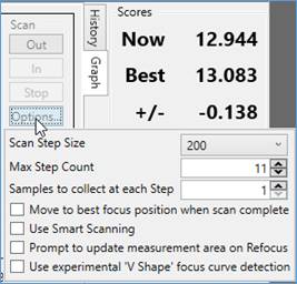
The details of the focus scan can be configured by pressing the Options… button and setting

· Scan Step Size – this is the amount of focuser movement between each focus measurement

· Max Step Count – this is the total number of steps of Scan Step Size to make during the focus scan

· Samples to collect at each Step – the number of focus score samples to use to measure the focus score at each step. Note that SharpCap will wait at least one frame to allow movement to settle at each step before starting measurement.

Note that if you have set an averaging option (perhaps to 5 frames) and you set 3 samples here then 15 frames 5*3 will be collected at each position.

· Move to best focus position when scan complete – when this option is selected and a focus scan successfully determines the point of best focus, SharpCap will automatically move the focuser to the best focus position after the scan finishes.

· Use Smart Scanning – when this option is selected, SharpCap may modify the scan to try to ensure success of the focus scan. This can include adding extra steps to the end of the scan if success seems likely but not enough data has been collected to be sure. Additionally, SharpCap may stop the scan early if a best focus position has clearly been found before the specified number of steps is complete

· Prompt to update measurement area on Refocus – enabling this option will cause SharpCap to pause to allow the Selection Area to be positioned correctly when running a Refocus. This is most useful when focusing for the sun, moon or planets.

· Use experimental ‘V Shape’ focus curve detection – SharpCap usually looks for a ‘U’ shaped pattern in the focus data, which works well when close to focus. Enabling this option makes SharpCap look for a ‘V’ shaped pattern instead, which may help if the scan includes data from a considerable distance out-of-focus on each side of the best focus position.

Automatic focusing with a Bahtinov Mask

The discussions of automatic focussing above concentrate on focus score methods such as Contrast Detection and FWHM Measurement which give either a maximum value or minimum value at the point of best focus. When using the Bahtinov Mask focus tool, the best focus is at the point where the focus score is zero.

The automatic focussing routines described are capable of working with the Bahtinov mask tool and will properly return to the point where the focus score is zero.

ASCOM Focusers and Backlash

Backlash in the focuser mechanism will be present in all real focusers and shows itself as the best focus point appearing in differing positions depending on which direction the focuser is moving.  So, if the peak focus score is at focuser position 20100 when the focuser is moving in the positive (+ve) direction, it could be at 19900 when moving in the negative (-ve) direction, there are 200 steps of backlash in the focuser movement.  If trying to return the focuser to the position where the score was at its best, always approach from the same direction used when measuring the focus to avoid errors caused by backlash.

Ideally, you should calculate the amount of backlash in your focuser (the difference between the best focus position in the positive and negative directions) and configure SharpCap to correct for that amount of backlash. See Focuser configuration.

Fully Automatic Focusing

Fully automatic focusing (for deep sky images) is available via the Refocus button and also the Sequencer and the Deep Sky Sequence Planner. Fully automatic focusing builds on the scan and return to best position steps described above, so it is best to ensure that those steps work correctly before using fully automatic focusing. Note that fully automatic focusing is a SharpCap Pro feature.

The Refocus Button

The Automatic Refocus button is available in the Focus Assistant sub-menu and in the focus tools dropdown in the toolbar. An almost equivalent Refocus button is available in the Focus work area.

To use these options to perform a refocus, the following conditions must be satisfied:

· A camera must be open

· An ASCOM focuser must be selected and connected

· A previous focus scan and goto the best focus position must have succeeded

· A SharpCap Pro license is required

When a focus scan succeeds in finding the point of best focus, SharpCap saves information about the settings used for that scan – number of steps, size of each step, number of samples captured at each step, which focus tool was used, etc. These saved settings are re-used by the Refocus tool. Note that the Automatic Refocus buttons will launch the same focus tool (i.e. Multi-star FWHM or Contrast (Edge) detection) that was used for the previous successful focus, where the Refocus button in the focus work area will use the currently selected tool.

When Refocus is in progress, the main SharpCap user interface will be disabled to prevent manual adjustments to camera settings or focuser position from interfering with the automatic focus procedure. A Refocus Progress window will be shown, which gives updates on the current status of the refocus operation.

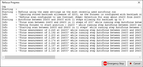
The focus work area will also appear, showing the focus data as it is collected on the graph tab. Any data previously showing in the focus graph area will be cleared at the beginning of the scan to ensure that only data from the scan is included in focus measurements.

The Refocus Progress window has both the Cancel and Emergency Stop buttons to allow the procedure to be stopped if necessary.

· The Cancel button will stop the scan as soon as possible and will return the focuser to the position it was in before the scan started.

· The Emergency Stop button will stop the scan straight away and will also send ‘stop movement’ commands to the focuser and any other connected ASCOM hardware. The focuser will not be returned to the initial position. This button can be used when something seems to be going wrong and you are concerned that hardware damage may occur if the procedure continues.

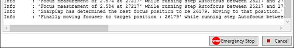
If the refocus procedure is successful in finding the point of best focus then the results of the calculation will be shown in the progress window and the focuser will be moved to the point of best focus. The Refocus Progress window will close automatically a few seconds after the refocus process is completed.

If the refocus procedure fails then information about the failure will be shown in the progress window, the focuser will be returned to the initial position and the progress window will close after a few seconds. An error notification will also be shown giving the reason for the refocus failure.

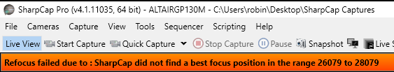
Note that if the Refocus procedure opened the focus work area then it will close it again at the end of the refocus run. If the focus work area was already open when the refocus was started then it will remain open after the end of the refocus run.

Refocusing from the Sequence Planner and Sequencer

When using the Deep Sky Sequence Planner, autofocus and refocus will be performed using the Multi-star FWHM tool. Additionally, the range of the refocus scan (how many focuser steps either side of the current position) and the number of measurement steps to take within that range can be specified manually. The values to use for these settings should be reasonably easy to choose once you have some experience with focus scans and the use of the Refocus button. Progress of the focus procedure will be displayed in the main sequencer progress window, but otherwise the procedure runs in a similar manner to the Refocus procedure described above.

When using the sequence editor, three autofocus steps are available for use

· Autofocus between <Start Focuser Position> and <End Focuser Position> with <Scan Step Count> steps allowing for backlash of up to <Backlash Allowance>

· Autofocus from offset <Start Focuser Position (Offset)> to <End Focuser Position (Offset)> with <Scan Step Count> steps allowing for backlash of up to <Backlash Allowance>

· Refocus using the same settings as the most recently used autofocus run

The first two steps will always use Multi-star FWHM and allow the range and number of measurement steps to be specified in the same way as in the Deep Sky Sequence Planner. The second option specifies positions relative to the current focuser position, while the first specifies absolute start and end points.

The third option is identical in effect to using the Automatic Refocus option from the menu or toolbar, as described above.

Setting the Correct Black Level

For most focus score tools, setting the correct Black Level value will help give more reliable scores. Parts of the image that are below the Black Level brightness are not included in the focus score calculation. Note that the Multi-Star FWHM score does not require the black level to be set manually – it is handled automatically.

Before setting the black level, ensure the object is not over-exposed by viewing with the Image Histogram – avoid the Image Histogram hitting the right-hand side.

For a large planetary target, the optimum black level is when there is a thin black area between the object and the dark area.  This can be difficult to see, so use the Zoom tool from the tool bar to improve the detail.

Contrast (Edge) Detection focus score used. Here the Zoom is 100%.  The black level happened to be 6.5% in this case. The actual optimum percentage black level will vary depending on camera and settings.  The picture illustrates how the black level shading should look when the black level is set correctly.

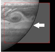
When the ROI is over the planet, and everything within the ROI is part of the desired image.  The requirement is to measure the focus of all of it.  Hence in this case, the black level is set to low or zero.

For a star as target, the optimum black level is when there is a thin black area between the object and the dark area.  This can difficult to see, so use the Zoom tool from the tool bar.

FWHM focus score used. Here the Zoom is 150%.  The black level happened to be 21% in this case. The actual optimum percentage black level will vary depending on camera and settings.  The picture illustrates how the black level shading should look when the black level is set correctly.

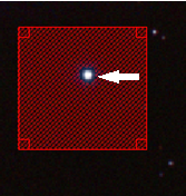
This is the effect of the correct black level on the focus score, making it clear the graph should always be reset after adjusting the black level or other parameters to avoid confusing the results of these adjustments with actual changes in the quality of focus.

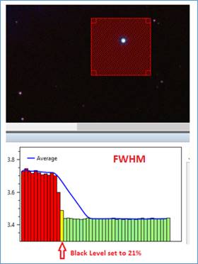
Using a Bahtinov Mask

A Bahtinov mask must be fitted to the telescope for the Bahtinov mask focus score tool to work.  Here are examples of diffraction patterns obtained using a Bahtinov mask in the conventional way, where the intersection of all three diffraction spikes at a single point indicates good focus.

Good	Off to the left	Off to the right

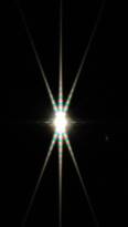
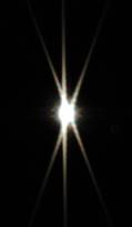
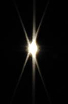
The Bahtinov Mask is used for single stars, which must be selected with the region selection area. Good focus is indicated by short green bars.  No bars, or a score of 0, indicated perfect focus.

When using the Bahtinov mask tool, ensure the Black Level control is set to a value that excludes the background area around the diffraction spikes from the focus score calculation but includes the entire visible diffraction spike area.

SharpCap attempts to detect the diffraction lines created by the Bahtinov mask and calculate whether they all meet at a single point (in focus) or not – SharpCap will draw coloured lines over the diffraction spikes as can be seen in the diagrams below.

Check the lines really are following the diffraction spikes, as sometimes the wrong lines will be detected and if this happens (as shown in the diagram on the right) the focus score will not be accurate.  When the lines are detected incorrectly, it is usually possible to correct the problem by adjusting the black level or camera parameters such as gain or exposure.

Diffraction spikes	SharpCap overlay	Resulting graphic
Diffraction spikes overlaid by the SharpCap mask gives the aligned graphic at focus.

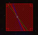
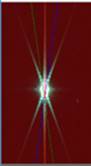
Live Stacking

Live stacking is a feature that enables the capture of deep sky images within SharpCap without the traditional requirements of a high accuracy, guided, equatorial mount and long sub-frame exposures.  The capture of a larger number of shorter exposures and software correction within SharpCap for any drift or rotation of the field of view between frames makes deep sky astrophotography accessible to a much wider audience at much lower cost.

The traditional requirements of long exposures and accurately guided mounts arise from traditional CCD cameras used for deep sky astrophotography have a high-level of read noise.  If there is a high read noise every time that a frame is captured, long exposures are required to allow faint deep sky objects to be seen above the read noise level.  Long exposures mean that an equatorial mount which tracks accurately and is typically auto-guided is required.

This all changes when modern low noise CMOS cameras are used instead of CCD cameras.  The low level of read noise means that faint objects can be detected in far shorter exposures (and can be enhanced by stacking many short exposures – something that would not be possible without low read noise).  If exposures are short enough (often 30s or less), mount accuracy is less important as the amount of drift during a 30s exposure is far smaller than the drift during a 300s exposure.  Away from the zenith, field rotation due to the use of an ALT/AZ mount is also not usually going to be significant during a single 30s exposure. SharpCap corrects for any gradual drift or rotation between successive frames by tracking the movement of the brightest stars in the image.  As the number of frames captured increases the noise level visible initially visible in the stacked image will reduce giving astounding deep sky images with the minimum of fuss.

Because of the simple satisfaction of watching deep sky images appear in real time without the need to use a separate stacking program, Live Stacking is particularly well suited to outreach uses.

Live Stacking is started by choosing the ‘Live Stack’ option from the Tools menu or by selecting the Live Stack toolbar button.

Once selected, Live Stacking will immediately begin capturing, aligning and stacking frames.  A minimum of 3 stars must be detected in each frame for alignment to be possible (see the following sections for further details on alignment and how to customize star detection).  It is possible to save the stacked image at any point using the Save button that appears in the Live Stack work area – the Save can be repeated as required – for instance after 50 frames and again after 100 frames and so on.

Note that adding more frames when using Live Stacking does not, by itself, make the image brighter (if you wish to make the image brighter, adjust the stretch applied in the Histogram tab or by using the Display Histogram Stretch). Instead, as more frames are added to the stack, the noise in the image will slowly reduce, producing a higher quality and more pleasing image. As the noise level reduces, you may find that you can enhance the image further by :

· Increasing the amount of stretch applied to brighten faint detail by using the Histogram tab

· Using sharpening adjustments in the Enhancement tab

These adjustments may give good results when the noise level is lower after many frames have been added to the stack, even if they look unnatural when there is a high noise level after only a few frames have been added to the stack.

The images below show the Horsehead Nebula after 1 frame (left), 10 frames (centre) and 100 frames (right) with otherwise identical settings for camera, live stacking and display stretch.

Working with Live Stacking

The UI to control Live Stacking appears in the work area below the camera image, and is divided into an always visible left panel and a series of tabs to the right.

The left panel controls and reports on the most important aspects of the stacking process and is always visible during Live Stack.  The right panel has ten tabs to allow the monitoring and control of the details of the Live Stack process.

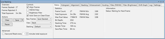
Left Panel

The most important controls in Live Stacking are located in the left panel and are available at all times – these include clearing and saving the stack and controlling key features such as alignment, filtering and whether to save raw frames.

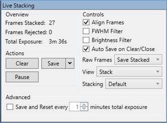
Overview Group

· Frames Stacked – the current number of frames on the stack.

· Frames Rejected – the number of frames rejected (not stacked).  This can happen because of alignment problems, SharpCap not seeing enough stars, frame failing to achieve a focus score criteria or other reasons.

· Total Exposure – the length of time the current stack has been running.  Some cameras cannot report their exposure value to SharpCap (for instance DirectShow Frame Grabbers).  In those cases, SharpCap estimates the exposure based on the time between subsequent frames.

Controls Group

· Align Frames – turn alignment and de-rotation on/off (default on).  See Alignment tab on right panel for more details.

· FWHM Filter – enable/disable filtering of each frame by the average FWHM (focus quality) value.  High FWHM value frames are discarded as indicating poor focus/seeing/transparency/cloud.  See Filter tab.

· Brightness Filter – enable/disable filtering of each frame by the brightness of the stars detected in the frame. A reduction in star brightness is often caused by thin cloud.

· Auto Save on Clear/Close – enable/disable saving the stack automatically when the clear button is pressed or another action causes the stack to be reset.

· Raw Frames – these options control whether the raw (unprocessed frames) are also saved. The options available are:

o Save None – Raw frames are not saved

o Save Stacked – Raw frames that are added to the stack are saved, frames that are not added to the stack are not saved (frames may not be added for a number of reasons : failure to align, FWHM or brightness filters, stacking being paused, dithering)

o Save except when Paused/Dithering – Raw frames are saved except when the stacking has been paused or when a dither operation is taking place

o Save All – All raw frames are saved.

Note that the saved raw frames do not have any pre-processing applied to them (dark subtraction, flat correction, banding suppression or background subtraction, etc.). This means that they can be processed later in another application.

Note also that the Preferred Still Format setting will determine the file format that the raw frames are saved to, and the raw frames will be found in a folder like YYYY-MM-DD\Capture\HH_MM_SS\rawframes.

· View – you can choose to view either

o Stack (show the stack so far – the default)

o Individual Frames (show the individual frames being captured by the camera). This can be useful when you are having problems with live stacking. By viewing the individual frames, you can see what stars are visible, if conditions have changed, etc.

· Stacking – Allows you to choose the stacking algorithm between the default algorithm, the sigma-clipping algorithm and the maximum value (meteor detection) algorithm. See Stacking Tab for more details. Note that changing the stacking algorithm will reset the stack.

Actions Group

The Clear button will reset the stack to start from scratch.  Note, other actions can cause the stack to be reset; for instance, changing camera, resolution, colour space, etc.  Changes to exposure, gain, brightness or applying a dark/flat will not cause the stack to be reset, but such changes should generally be avoided while a stack is in progress as they may lead to poor results.

The Save button has 4 sub options:

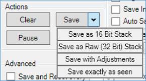
· Save as 16 Bit Stack will rescale the stacked data linearly between the 0 and the maximum pixel value into the range 0 to 65535 and save this as a 16-bit FITS file.  The 16-bit FITS option is the default as it gives a high bit depth image with the full range of the image used (i.e. brightest pixel is 65535).

· Save as Raw (32-bit) Stack will save the full 32-bit stack data as a 32-bit FITS file.  The data will be bit-shifted to fill most of the available range of 32-bit data (the amount of bit-shifting will be stored in the BITSHIFT header of the fits file).
Note: when using Sigma Clipped stacking, the 32 bit values will be stretched up to a maximum value of 2³¹-1.
Note: SharpCap can be configured via the Saving Settings to Save 32 bit FITS files as Floating Point. This can increase compatibility of these saved files with some imaging/processing applications such as GIMP.

· Save with Adjustments will save the image with the Live Stacking adjustments applied (i.e. after histogram adjustments and colour adjustments have been applied) as an 8 or 16-bit PNG file (depending on bit depth of camera being used).

· Save Exactly as Seen will save the image exactly as shown on screen as an 8-bit PNG file. This will include the effects of both the live stacking histogram and colour adjustments and the display stretch if one is applied.

The Pause/Resume button will temporarily stop or resume stacking.  Stacking will automatically be paused if the Live Stack window is closed or if the user switches to another tool such as Histogram. Switching back to Live Stack will allow stacking to be resumed in these circumstances if another action would cause the stack to reset has not been carried out (for instance changing resolution or colour space), providing that live stacking has been closed for less than 60 seconds. This ensures that stacked data is not lost through accidentally selecting other SharpCap functions that might close Live Stacking.

Finally, in the Advanced section, you can choose to automatically save and reset the stack after a selectable interval. This can be useful if you live in an area with heavy aircraft traffic as taking a large number of shorter stacks may avoid a single set of aircraft lights spoiling a long stack. Note that the time limit for this depends on the Total Exposure for frames added to the stack, so the actual time may be longer if frames are rejected or actions such as dithering interrupt stacking.

Status Tab

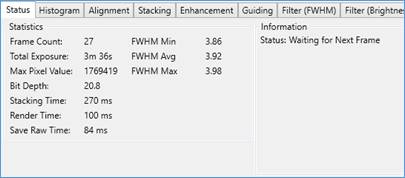
The Status tab shows some more detailed information about the stacking process and the stack so far.  Of interest is the Stacking Time, which is the amount of time taken to process the alignment and stacking calculations needed for each frame.  If this time is longer than the exposure length, frames will be dropped from the stack (due to the previous frame still being stacked when the next frame arrives).  The Render Time indicates how long the calculations to redraw the image on screen take to complete. Certain Live Stacking features such as noise reduction and sharpening can increase the render time. If the render time is large then the program will only respond slowly to changes in the Live Stack histogram or colour settings. The Save Raw Time shows how much time is being used saving raw frames to file (if that option is enabled).

The right-hand column of the Statistics shows information on the FWHM measurements made on frames captured during the stack so far, showing the FWHM values of the best (minimum) and worst (maximum) frame as well as the average frame FWHM. Note that if the FWHM Filter option is enabled, some of the frames with higher FWHM values may have been excluded from the stack by the filter.

The right-hand information panel shows the current status or warning or error messages if stacking errors are occurring.

Histogram Tab

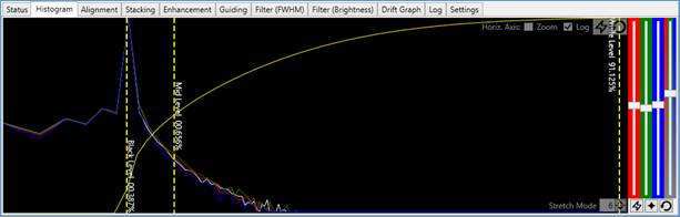
The Histogram tab shows not only the histogram of the live stack data, but also allows the image levels to be stretched by moving the three vertical dashed yellow lines which represent the White Level, Black Level, and Mid-Level. The yellow curve shows the Transfer Curve which determines how bright the viewed image is for a given histogram level. For pixels at the Black Level point (and below) the viewed image will be black. For pixels at the Mid-Level point the viewed image will be mid (50%) grey. For pixels at (or above) the White Level point, the viewed image will be at maximum (100%) intensity.

· Tweaks to the Black Level, White Level and Mid-Level affect how the image is shown on screen and how it is saved if choosing Save with Adjustments or Save Exactly as Seen. 

· The changes do not affect the actual values in the stack or the result if Saving As 16 or 32 bit stacks. 

· Changes made to the levels here do not affect the shape or position of the histogram shown in the Live Stacking panel, but will show in the Mini Histogram in the Camera Control Panel on the right.

· Additionally, the Histogram Stretch Controls on the right, in the Camera Control Panel, affect only how the image is viewed on screen and do not affect saved data except when using the ‘Save Exactly as Seen’ option. 

Adjust White Level

· The white level applies to the horizontal axis of the histogram, so left is 0% and right is 100%. It is not usually necessary to adjust this line.

Adjust Black Level

· The black level applies to the horizontal axis of the histogram, so left is 0% and right is 100%.

· Turn up the Black Level slightly (move slider to right) to suppress sky glow/chip noise and give a dark background to an image.  Turning the black level up too far can give the image an unnatural look or make faint detail vanish.

Adjust Mid-Level

· The mid-level line also applies to the horizontal axis of the histogram and specifies the level on the histogram that will be displayed as a mid (50%) grey level. The mid-level is restricted to be between the black level and the white level.

· Moving the mid-level control to the left towards will enhance the brightness of dim areas of the image. Moving the mid-level control to the right towards the white level will darken dim areas of the image but enhance contrast in the brighter areas of the image.

Transfer Curve

· The yellow transfer curve shows how the levels between the black and white points are going to be displayed on screen.  The shape of this line is determined by the positions of the black level, white level and mid-level controls, and the line acts in a way similar to the ‘Curves’ adjustment found in many image processing applications.  For this line the vertical axis of the graph is the display brightness from black (bottom) to white (top).  The brightness of a pixel in the viewed image is calculated by taking its horizontal position of the pixel on the histogram, moving up to the red transfer curve line and taking the vertical position of the line at that point as the displayed brightness for that pixel.

Auto-Stretch and Reset Buttons

These buttons are located at the top-right of the main histogram area. The Auto-Stretch button (with the lightning bolt) will automatically set the black, mid and white levels to appropriate values to enhance the view of the image being stacked. The Reset button (with the circular arrow) will set the levels back to their default values. Note that the use of the Auto-Stretch button requires a SharpCap Pro license.

If you find you want a slightly stronger stretch, hold down the CTRL key while clicking on the Auto-Stretch button. Holding down the SHIFT key will give a slightly weaker stretch than normal. You can also adjust the strength of the default stretch in the Display Settings.

Colour Adjustment

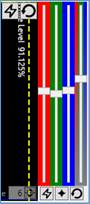
The colour adjustment sliders can be found to the right of the main histogram area and only show for colour cameras. The four sliders are, in order from left to right:

o Red Adjustment

o Green Adjustment

o Blue Adjustment

o Saturation Adjustment

The three colour sliders can be used to adjust the colour balance of the image. The saturation slider can be used to increase or decrease the amount of colour seen. Adjustments made here affect the image as viewed on screen and the saved images when choosing either ‘Save With Adjustments’ or ‘Save Exactly as Seen’.

The colour adjustment sliders can apply an adjustment of between -10db (0.32x) and +10db (3.2x) to each colour channel.

Below the colour sliders are three buttons – from left to right:

o Auto colour balance based on aligning image histogram peaks

o Auto colour balance based on star colours

o Colour adjustments reset button

Horizontal Axis Scaling

The scaling of the horizontal axis of the histogram can be adjusted by checking one or both of the Zoom and Log(arithmic) checkboxes.

Using either the horizontal axis zoom or the logarithmic scaling can make it much easier to adjust the histogram (particularly for faint targets), since it makes the region of interest in the histogram take up much more of the available space.

Stretch Mode

Adjusting the Stretch Mode provides additional control over the shape of the transfer curve, which may be useful when imaging some targets. In particular, bright targets such as M31 or M42 may be difficult to adjust correctly in the default stretch mode (mode 2), giving over-saturated bright cores. Setting a higher Stretch Mode increase the steepness of the transfer curve in the darker regions of the histogram and reduces the steepness in the brighter regions, which may help deal with bright targets.

Note that in higher stretch modes, it may be difficult to adjust the black level correctly in the Live Stack histogram, however the Display Histogram Stretch control allows these fine corrections to be made easily in this situation.

Making fine adjustments to the Histogram

Sometimes it is necessary to make fine adjustments to the histogram stretch levels or the colour balance sliders to get the desired effects.

· Hold down the <SHIFT> key while dragging the Black/Mid/White level lines – this will reduce the speed at which the lines move, making them easier to adjust.

· Start dragging the Black/Mid/White level lines and move the mouse pointer to the top of the screen while continuing to drag. The further you move the mouse pointer out of the histogram area, the slower the lines will drag left/right

· Click on one of the colour balance bars and use the up/down arrow keys on the keyboard to make small adjustments or make the live stack area taller.

· Tick the Logarithmic Horizontal Axis checkbox, which will adjust the horizontal scale of the histogram to give more space to the shadows and mid-range and less to the highlights region. Note that the vertical scale of the histogram is always logarithmic.

· Holding down <SHIFT> while adjusting the colour balance and saturation sliders also provides fine adjustment, with the adjustment made being reduced by about 10 times from normal.

Alignment Tab

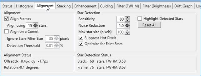
The Alignment tab controls the alignment process which, along with the FWHM filter, depends on the detection of stars in each image.  SharpCap can only align images in which it can detect stars (do not use Live Stack for planetary, solar or lunar images).

· A minimum of 3 stars is required for Live Stack with alignment to work.  However, for reliability and good alignment a star count of 10-15 or more is to be preferred.

· Too many stars being detected can also cause problems, with either false alignment matches or with the star detection stage slowing down the stacking process. 100 to 200 stars is sufficient.

Alignment Group

· Align Frames – enable or disable the alignment of frames.  The first frame in any stack becomes the reference frame – all other frames are aligned with that frame when alignment is enabled.  SharpCap uses the stars it detected in the first frame to align all subsequent frames with the stack.  Stars in the stack are re-detected if any of the star detection parameters are changed.  The absolute minimum requirement is 3 stars detected, although having 3 stars is no guarantee of alignment working if too close together or close to being in a straight line for instance.  Ideally, aim for 10-20 or more stars detected with a good distribution across the frame.

· Align using – to select number of stars.  It can be 10, 15, 20 or 25 stars.  Using a larger number of stars may slow down the stacking process, but may give better alignment results. Only increase this value if detecting plenty of stars but still having difficulty aligning.

Comet Alignment

· Align on a Comet – enabling this option changes the alignment calculations to a mode where aligning on a comet is possible. Instead of using 3 or more stars to align, in Comet mode, SharpCap looks for a single fuzzy blob in the image and aligns on that. Since the comet is likely to be moving appreciably against the background stars, the stars will form trails in the resulting image, but the comet should form a good image. The image below shows comet C2022/E3 (ZTF) captured in Live Stack Comet mode.

· Ignore Stars Filter Size – when aligning on a comet, SharpCap needs to ignore all the stars in the image (which are small and bright) so that the only bright thing left is the comet (which is more spread out and bright). As SharpCap processes the image looking for the comet, it will wipe out stars up to the size specified by this setting. Note that a second extended object in view (galaxy, nebula) may confuse the comet alignment routines and should be avoided.

· Detection Threshold – with the stars removed according to the Ignore Stars Filter Size, SharpCap will look for the brightest area of the frame (the brightest pixels as limited by this threshold) and use the average position of those bright pixels as the position of the comet.

Comet alignment is best set up by

· Turning on Align Frames and Align on a Comet

· Turning on Highlight Detected Stars

· Switching the View option to Individual Frames

· Setting a good Display Histogram Stretch to make the comet visible in the individual frames

In this configuration, SharpCap will highlight a single ‘detected star’ in the image – the place it is detecting for the comet. Now adjust the Ignore Stars Filter Size and Detection Threshold until the detected position aligns well with the nucleus of the comet. In general a high Ignore Stars Filter Size and a low Detection Threshold give good results.

Note that Comet Alignment is a SharpCap Profeature.

Once the detection rectangle is aligning with the comet nucleus, turn off Highlight Detected Stars, switch the View option back to Stack and reset the stack to start a new comet stack that should align correctly.

Because comet alignment depends on detection of a single target (the comet), it cannot adjust for rotation of the image as normal star based alignment can. Avoid using comet alignment with an Alt-Az mount (particularly near the Zenith) otherwise the stacked image quality may be affected by rotation.

Star Detection Group

· Sensitivity – This controls the overall sensitivity of the star detection process – increase this value to try to detect more stars, decrease it to reduce the number of stars being detected. Note the following:

o Setting a higher sensitivity can make star detection take longer, potentially slowing down the stacking process

o SharpCap will auto-adjust the sensitivity for you, turning it down (to a minimum of 75) if more than 200 stars are detected and turning it up (to a maximum of 75) if less than 25 stars are detected.

· Noise Reduction – when enabled applies a Gaussian blur to help SharpCap to ignore low level noise and hot pixels.  Increasing this may help detect stars correctly in noisy images.

· Maximum Star Size (pixels) – set a maximum star size, which can be helpful to prevent SharpCap from detecting small non-stellar targets (such as Planetary Nebulae) as stars.

· Suppress Hot Pixels – Enabling this option adjusts the star detection process to avoid detecting a star from a single hot pixel in the image. You may need to turn this off if you are using a large pixel camera and a short focal length telescope (i.e. your stars are very small).

· Optimize for Faint Stars – Use this option if you are having trouble with alignment but can see faint stars in the image that are not being detected.

· Highlight Detected Stars – checking this will put boxes around the detected stars – yellow stars are used for alignment; red are not used for alignment.  This can be very helpful to determine and understand the causes of problems with star detection and alignment.

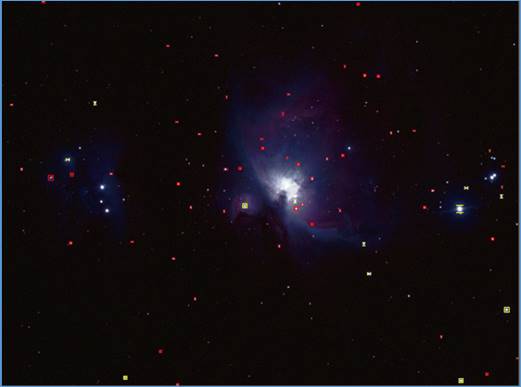
Note that the detected stars shown are the stars for the stack when View is set to Stack, and are the stars for the raw frames from the camera when View is set to Individual Frames.

· Reset All – this button resets all star-detection related options to their default values.

Status Groups

· Shows various data including offset of the frame from the stack, rotation and number of stars detected. 

Note that the offset and rotation is relative to the first frame in the stack.

Stacking Tab

The Stacking tab allows the selection of either the Default or Sigma Clipped stacking algorithm and also allows adjustments to be made to the settings for the Sigma Clipped algorithm.

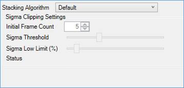
Default Stacking

The Default Stacking Algorithm adds the pixel values from each frame to the stack data. All frame date from stacked frames is included in the stack. The default stacking algorithm does not have any adjustable controls.

Sigma Clipped Stacking

The Sigma Clipped Stacking Algorithm averages stacked frames together to create the stack data. The algorithm tracks fractional pixel values, so stack quality is maintained. The algorithm also compares the value of each pixel in a new frame to the value of that pixel so far in the stack – if the two differ too much the data from that pixel is ignored for that frame.

The advantage of Sigma Clipped stacking is that anomalous features in individual frames – for example satellite or aeroplane trails do not end up in the stack data, since the anomalously bright pixels are rejected by the algorithm.

SharpCap keeps track of the mean value of each pixel in the stack as well as the amount of variability in the pixel value for each pixel. The amount of variability for each pixel is known as the standard deviation or Sigma value for each pixel.

The decision on whether to include the data for a particular pixel from a particular frame in the stack is made on the basis of the difference between the pixel value in the frame and the mean pixel value in the stack so far for that pixel. The size of this difference is compared to the sigma value for that pixel multiplied by the Sigma Threshold value. If the difference is larger than the pixel data is ignored.

The following controls are available to adjust the behaviour of the Sigma Clipped Algorithm:

· Initial Frame Count – this controls the number of initial frames during which the algorithm learns what values are expected for each pixel without rejecting any potentially unusual values. A value in the range 5 to 10 is usually sufficient.

· Sigma Threshold – this controls how different from the current stack pixel value a frame pixel value must be to be rejected. Setting a higher value here will mean that less pixel data is discarded but will reduce the effectiveness of the algorithm at excluding anomalous pixel data. This control should be adjusted while watching the Status information which shows the fraction of pixels being rejected in each frame.

· Sigma Low Limit (%) – this control specifies a lower limit on the value of sigma calculated for any pixel in the stack. This is required to prevent incorrect rejection of image data when the individual frames have very little noise.

Note that Sigma Clipped Stacking requires a SharpCap Pro license.

Maximum Value (Meteor Detection) Stacking

When the stacking mode is set to Maximum Value (Meteor Detection), SharpCap will use the maximum pixel value seen at a location as the value to be displayed (rather than the average value as used in other modes). In this mode, stacking will not reduce image noise significantly, but meteor trails across the image (and satellite trails for that matter) will persist rather than slowly fading due to averaging.

Enhancement Tab

The controls in the Enhancement tab provide a way to improve the live stack image by either reducing the noise in the image, sharpening the image or both. All tools in the enhancement tab, except for the simple Gaussian Blur noise reduction require a SharpCap Pro license.

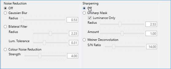
Gaussian Blur – a simple noise reduction tool which blurs each pixel in the image with its neighbours. This helps reduce the noise in the image but also has the effect of blurring the image somewhat. The Radius control determines how large an area each pixel is blurred over, increasing this value will strengthen the noise reduction effect but also blur the image more.

Bilateral Filter – a more sophisticated noise reduction tool which can reduce noise in areas of similar colour without blurring detail as much as the Gaussian Blur noise reduction tool. Once again, the Radius control determines the area over which the noise reduction operates. The Luminance Tolerance control determines how big a change in brightness is required to be regarded as a feature that will be preserved. The Bilateral Filter algorithm requires much more calculation than the Gaussian Blur algorithm and may slow down live stacking when using high resolution cameras or on slower computers.

Colour Noise Reduction – a noise reduction applied only to the colour information in the image (to be precise to the Cb and Cr channels of the image in YCbCr format). This can be particularly effective in reducing the apparent noise in an image in the early stages of stacking when only a small number of frames have been stacked. Because no noise reduction is applied to the luminance channel, fine detail in the image is largely unaffected.

Unsharp Mask is a simple image sharpening tool which strengthens the sharper components of the image relative to the less sharp components, producing a sharper looking image. The Radius control adjusts the split between the ‘sharp’ and ‘less sharp’ components of the image – the higher the value set the larger the scales of details that will be considered part of the ‘sharp’ component. The Amount control determines how much boosting is applied to the ‘sharp’ components of the image. Applying the Unsharp Mask sharpening unfortunately has the side effect of increasing image noise in the image. Setting the Amount control to too high a value may lead to an unnatural look to the image.

Note that for colour images it is possible to apply the Unsharp Mask sharpening only to the luminance of the image by ticking the Luminance Only checkbox. This can be helpful to avoid the creation of colour artefacts in the image when sharpening.

Weiner Deconvolution is a sophisticated image sharpening tool based on determining the shape of stars in the stacked image as an indication of the nature of blurring in the stacked image, then attempting to undo this blurring to the image to produce a sharpened image. The only control to adjust for this sharpening algorithm is the Signal to Noise Ratio. This is an estimate of how much brighter the image signal is in the stack than the noise. The Signal to Noise Ratio control should be set to the highest value that gives a natural look to the image (setting the value too high will give the image an unnatural, ‘orange peel’ look). The Weiner Deconvolution algorithm requires a significant amount of calculation and may slow down live stacking when using high resolution cameras or on slower computers.

Note that Weiner Deconvolution requires star detection to be active and finding stars in the image, since it uses the average star shape as an estimate of the ‘Point Spread Function’ which describes how the image has been blurred by seeing, optics, etc. If no stars are being detected then the deconvolution option will have no effect. Weiner Deconvolution is only applied to the luminance channel of colour images.

The sharpening and noise reduction algorithms affect both the image as shown on screen and the image saved when using Save with Adjustments or Save Exactly as Seen. Since the sharpening and noise reduction is applied every time the image on screen is updated, using these tools may reduce the responsiveness of the live stacking to changes in other controls such as colour adjustment or histogram changes.

Guiding Tab

SharpCap can work with the popular freeware guiding application PHD2 and also the MGEN3 Autoguider to monitor and control guiding and dithering while live stacking. Additionally SharpCap can dither using a connected ASCOM mount without needing a guiding application. See the Guiding Settings for more information on configuring guiding/dithering options, including configuring dithering settings that were found in this tab in older versions of SharpCap.

The Guiding tab also allows you to set up periodic re-centring of the target using Plate Solving and a GOTO mount. This is an excellent way to prevent the telescope from drifting too far from the target if you are not guiding.

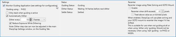
Configure your guiding setup in the Guiding Settings before trying to start guiding or dithering while live stacking.

If Monitor Guiding Application is checked then SharpCap will attempt to connect to the selected guiding application/device when live stacking starts. A notification message will indicate if connection has succeeded or failed and if connection succeeds then the Status information will update regularly.

If SharpCap has successfully connected to the guiding application/device then a status such as ‘Guiding’, ‘Calibrating’ or ‘Stopped’ will be shown in the Status box on the right. If guiding monitoring is disabled or SharpCap cannot connect to the guiding application/device then ‘Not connected to guiding’ will be shown.

To retry the connection (perhaps if PHD2 was not running initially, or your MGEN3 device was not plugged in), uncheck and then re-check the Monitor Guiding Application checkbox.

Monitoring Guiding

Basic guiding monitoring is managed by the following option:

Only Stack when guiding is active – if enabled then SharpCap will pause any live stack in progress if the guiding status changes from ‘Guiding’ to any other status, or if guiding is not connected. Note that if you start a new stack with this option enabled and guiding is not active, SharpCap will not stack any frames until the option is cleared or guiding becomes available.

Notification messages will be shown in the SharpCap notification bar when guiding starts or stops, explaining if stacking is disabled due to guiding not being active.

Note that if Dither Only Guiding is selected in the Guiding Settings then SharpCap will always report guiding as active if an ASCOM mount is available, and the Only Stack when guiding is active checkbox has no effect.

Dithering

SharpCap Pro users can also enable dithering using their guiding application/device while live stacking. In order to enable dithering, tick the Automatically Dither checkbox and set the dithering interval as required.

SharpCap will send instructions to dither at regular intervals. The dithering interval may either be set as an elapsed time (in seconds) between dither operations or as a number of captured frames between dither operations. If the dithering interval is set to a time and the dither time arrives while a frame is being captured, SharpCap will wait until the frame ends before starting dithering.

SharpCap will exclude frames captured during the dithering operation from the stack, so that frames that may be blurred due to the dithering movement are not included in the stack. The stack will recommence normal operation after the end of the first frame to finish after the dither has finished settling.

Dither Every – this specifies the interval between dithering operations, either in frames or in seconds. Note that if a short dither interval is specified (i.e. dithering every frame or two), it is critical to set the Reduce Exposure while Dithering option to avoid an unacceptable loss of time due to a large fraction of frames being discarded due to dithering.

Reduce Exposure while Dithering – If this option is selected then SharpCap will reduce the exposure of the camera to approximately 2 seconds during dithering operations and reset it back to the normally selected exposure time when the dithering operation is complete. This reduces the amount of lost imaging time at each dither and should normally be left checked. The reduced exposure (2 second) frames will not be added to the stack and will not be saved as raw frames unless the Save All option is selected for saving raw frames. The use of this option is recommended.

Automatic Recentering

Automatic recentring provides an alternative to guiding as a way to limit mount drift for long stacking sessions. Recentring is available if the following criteria are satisfied :

· A GOTO mount is available and connected

· A Plate Solving application has been configured in the SharpCap settings

· Either Monitor Guiding Application is unchecked (no guiding) or it is checked but Dither Only Guiding is in use (as opposed to real guiding such as PHD2 or an MGEN3 device).

The functionality is controlled by setting the amount of drift that is allowed before recentring is activated – this is controlled by adjusting the Recenter when drift exceeds <XX> pixels value.

When the drift of the current frame from the stack exceeds the threshold, SharpCap will

· Plate solve the stacked image

· Calculate the mount offset needed to make the mount point back at the stacked image from the plate solving information and the stacking offset

· Reduce the camera exposure if the Reduce Exposure while Dithering option is set

· Move the mount as required to bring recentre

· Wait for the mount to settle

· Restore the camera exposure time

· Resume stacking new frames

Subsequent recentre operations will happen when the offset again exceeds the threshold – however, subsequent operations will not require plate solving as the data from the first operation is re-used.

If the plate solving fails then SharpCap will retry up to 2 more times before showing a failure notification and automatically disabling recentring to allow stacking to continue anyway.

Note that it is possible to configure SharpCap to treat the drift threshold as counting un-binned camera pixels by ticking the Treat above value as un-binned pixels checkbox. When checked and using binning, SharpCap will for example treat a threshold of 40 pixels as being equivalent to 20 pixels movement at bin 2. This can be useful as it keeps the physical amount of drift allowed constant even if binning is changed.

Filter (FWHM) Tab

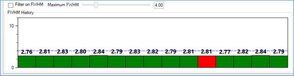
This filter allows poor-quality frames (poor atmospheric conditions or clouds) to be excluded from the stack.  Frame quality is judged only by the FWHM (full-width-half-maximum) estimate of the quality of focus in the frame.

· Filter on FWHM – check to enable FWHM (focus score) filtering.

· Maximum FWHM – use the slider to specify a maximum FWHM value for frames to be used.  It shows a history of recent frames.  Used frames are green, frames discarded by filtering are red.

· Filtering does not apply to the first frame in any stack.

Filter (Brightness) Tab

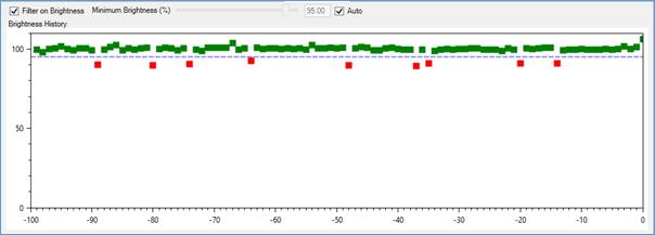
This filter can help detect reductions in frame brightness caused by passing cloud, stopping frames spoilt by cloud from being added to the stack. The frame brightness is judged based on the brightness of stars detected in the frame, so this filter can only operate correctly when sufficient stars are detected in the frame.

The graph shows the brightness of recent frames with the most recent frames on the right-hand side and the oldest frames on the left. Frames that are rejected are shown as red squares, frames that are stacked are shown as green squares.

The controls available are:

· Filter on Brightness – check to enable brightness filtering

· Minimum Brightness – adjust the level of brightness below which frames will be rejected. The level is measured relative to the average brightness of recently stacked frames.

· Auto – check this box to allow SharpCap to set the Minimum Brightness threshold automatically based on the statistics of recent frames. Uncheck this box to allow the Minimum Brightness to be set manually.

Drift Graph Tab

The drift graphs show the history of movement and rotation of the image during the current live stack.

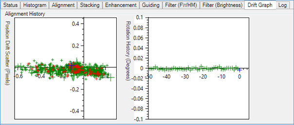
The left-hand graph shows the amount of movement of the image on a scatter (X,Y) graph. Green crosses represent frames that were added to the stack, red crosses represent frames that were not added to the stack for some reason (filtering, stacking paused, etc). More recent frames have larger crosses and the most recent frame is a blue cross.

The right-hand graph shows the history of rotation of the stack with the amount of rotation measured on the vertical axis and time (with the most recent frames on the right) measured on the horizontal axis. Rotation will be very low for equatorial mounts, but may be significant for Alt-Az mounts.

Hovering the mouse over either graph will display a larger version.

Log Tab

Shows some log information of Live Stacking in more detail than is saved in the main SharpCap log.  If something is not working, this is the place to look.

The log tab also contains two controls that are sometimes useful:

· Reset All Settings – pressing this button will reset all live stacking settings to their default values.

· Warn After X Ignored Frames – adjusting this setting changes the number of frames that must be ignored in a row before SharpCap begins showing warning notifications.

Settings Tab

The settings tab provides a number of options to customize the behaviour of live stacking.

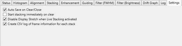
· Auto Save on Clear/Close – this duplicates the auto save option available in the Left Panel of the Live Stacking work area. When enabled, the current stack will be automatically saved if you Clear the stack or close Live Stacking. Note that auto-saving only occurs if at least one frame has been added to the current stack.

· Start stacking immediately on clear – when checked (which is the default), Live Stacking will begin stacking straight away with the first frame received from the camera after clearing the stack. When this option is disabled, clearing the stack will effectively pause Live Stacking – in order to start a new stack you must press the Pause/Resume button (which will change to a Start button).

· Disable Display Stretch when Live Stacking is activated – both the Display Histogram Stretch and Live Stacking contain can apply a strong stretch to the image to make faint detail visible. If you tend to keep the Display Histogram Stretch active to show faint targets when framing/slewing/focusing etc., you may notice that when you begin Live Stacking, the combination of the two stretches gives a poor result due to the displayed image being over stretched. By enabling this option, you can cause SharpCap to disable the Display Histogram Stretch when starting stacking (and re-enable it when stopping stacking) to avoid this problem.

· Create CSV log of frame information for each stack – SharpCap can create a log file with information about each frame considered for stacking. This feature is off by default, but can be turned on using this option. Note that the log is not saved unless at least one other file is saved from the stack (raw frame or saved using one of the save options). The information saved to the log includes :

o Date & Time that frame was captured

o Frame Index in the stacking process

o Whether the frame was added to the stack or not

o Number of stars detected in the frame

o Frame star brightness reading

o Frame average star FWHM value

o The offset of the frame from the stack in pixels (X and Y direction)

o The rotation of the frame relative to the stack

o The filename of the saved raw frame file (if saved)

Live Stack Reference

For default stacking, SharpCap maintains a 32-bit integer value for each pixel of the stack with the value from each frame being added to the pixel value.

· For a 16-bit camera it is possible to stack up to 32768 (2¹⁵) frames before running out of values in the stack.

· For an 8-bit camera it is possible to stack up to 16 million frames (2²⁴) before running out of values in the stack.

For sigma-clipped stacking, SharpCap maintains 2 32-bit floating point numbers for each pixel – to represent the average pixel value and the variation in the average pixel value.

All files saved during a stack will be saved in a single folder (raw frames and processed stack images saved in subfolders).  This helps keep the saves from the stack together.  The folder is named after normal file naming rules based on the time stacking was started and the name of the target object selected.

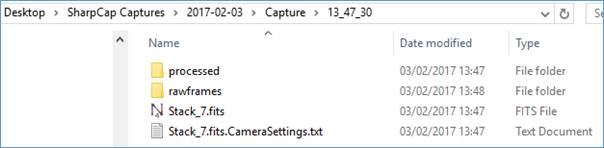
Renaming a Live Stack

If the name of the target in the toolbar is changed during Live Stacking, SharpCap will rename the output folder. This will take place automatically without prompting if no images have yet been saved by the current stack. If images have been saved then you will be prompted to confirm the rename of the stack.

Note: The live stacking process will be paused while waiting for the answer to the rename confirmation question.

Note: The new name is not applied until you click away from the Target Name box or use the <TAB> key to move the cursor out of the box.

Live Stacking with a camera in Still Mode

SharpCap can live stack with a camera that is in Still Mode (note however that you cannot change between Live Mode and Still Mode while Live Stacking is active).

When Live Stacking is enabled with a camera in Still Mode, SharpCap will automatically request frames from the camera as required to keep the stacking working – there is no need to use the Snapshot or Framing Shot buttons to capture frames.

There are some advantages to using Still Mode – when stacking is paused to allow for dithering, recentering or for other reasons, the camera can be kept idle rather than having it continually take frames as happens in Live Mode.

Seeing Monitor

The Seeing Monitor is a new application of the image quality measurement techniques that SharpCap has provided to assist focusing for some time. Instead of helping you find the point of best focus, you can now use the image sharpness measurements to help you capture the moments of clearest seeing without the eyestrain and fatigue usually associated with carefully watching the image to pick out seeing improvements.

Seeing Monitor is launched from the Tools Menu, and shows a chart of the recent range of image quality with the most recent values highlighted. This gives an objective measurement of when the seeing is at its best.

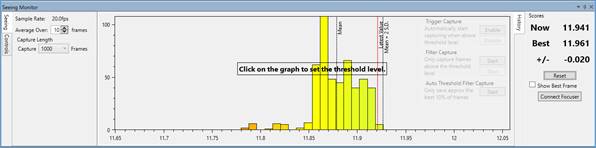
Every new frame is analysed for sharpness (contrast) and the results are added to the graph that will build up below the image. The quality of the results can be improved by selecting the area of interest using the selection area tool (for instance sunspots, prominences, craters). Using the standard colour scheme for focus measurements, sharp frames build the graph in green on the right hand side of the graph, poor frames build the left hand side in red.

If the seeing is relatively constant then the graph will be like the one above with a single peak. If the seeing improves or worsens then a new peak will begin to build (to the right for improved seeing, to the left for worse seeing), like the image below. Note that other factors can also change the score and cause a new peak – for instance brightening or dimming caused by passing thin clouds.

In both graphs you can see a number of vertical lines:

· Dashed line labelled Mean - The mean image quality value for all samples measured so far

· Dashed line labelled Mean + 2S.D. – The image quality value that corresponds to the mean plus two standard deviations. If the seeing is steady then you would only expect to see about 2% of frames exceed this level due to small random fluctuations.

· Solid red line labelled Latest Value – This shows the quality of the most recent frame recorded. If this line moves to the right of the Mean + 2SD line for any significant length of time then it is likely that the seeing has improved.

It is important to remember that other actions can cause the quality of the image to change – for instance

· Adjusting Focus

· Adjusting camera parameters such as gain or exposure

· Moving the selection area rectangle

· The image moving due for some reason (poor tracking, mount adjustments)

When any of these occur, press the Reset button to clear the graph and start accumulating new seeing data, otherwise the data may be misleading.

Configuring Seeing Monitor

On the left-hand side you will see a selection of controls allowing adjustments to be made to the Seeing Monitor settings.

· Sample Rate – shows how often SharpCap is measuring the frame quality

· Average Over <X> frames – controls how many frame measurements are averaged together before plotting a new data point on the graph. Typically this should be set to a value between one half and one fifth of the sample rate to give a few new data points being added each second

The options available in the Controls tab are identical in effect to those used for configuring the Focus Tools.

Finally, the Capture Length setting controls how many frames will be captured when a Seeing Triggered Capture begins – see below for more details.

Seeing Triggered, Seeing Filtered Capture

With a SharpCap Pro license, three additional functions become available – Seeing Triggered Capture, Seeing Filtered Capture and Auto Threshold Filter Capture. These functions help capture images when the seeing improves without the need to constantly watch the Seeing Monitor graph.

The first two functions (Seeing Triggered and Seeing Filtered Captures) rely on setting a Threshold level in the seeing monitor graph, which can be set and adjusted by clicking on any point in the graph.

Both modes can be activated using the buttons found on the right-hand side of the graph.

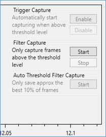
Seeing Triggered Capture will automatically start capturing when the Latest Value exceeds the Threshold Value and will then capture the number of frames given by the Capture Length setting in the left-hand controls region. Note that the specified number of frames will be captured even if the image quality then falls back below the Threshold level.

Seeing Filtered Capture works in a different way – when the Start button is pressed, SharpCap will immediately begin capturing, but will deliberately discard all frames where the frame image quality is below the Threshold Level. This will be reflected by the dropped frames count rising rapidly in the Status Bar. Only frames that meet or exceed the Threshold Level will be saved to the capture file. Capture will continue until the Stop Capture button on the toolbar or the Stop button is pressed.

Note: While Seeing Filtered Capture is active, the captured frame count shown in the status bar may seem to fluctuate slightly at times when all frames are being discarded. This behaviour is normal.

Note: Some frames may be saved to the output file even at times where the Latest Value line on the graph is below the Threshold line. This is because the position of the Latest Value line is an average of the image quality of a number of frames. The average value may be below the threshold, but a number of the individual frames that make up the average may have an image quality above the threshold.

Auto Threshold Filter Capture

Auto Threshold Filter Capture also utilizes the frame quality measurements to try to only save the best frames to file, but works in a different way – instead of setting a threshold manually, with this option, SharpCap can capture the best frames in a fully automatic way.

When capture is started using the Auto Threshold Filter Capture Start button, SharpCap will begin saving frames from the camera into memory, recording the quality information for each frame. When the memory storage becomes nearly full, SharpCap will automatically choose a quality threshold that will keep approximately 10% of the frames in memory and start saving those frames above the quality threshold and discarding the rest. At this point, memory levels will rapidly decrease and then the cycle of filling memory, choosing a threshold, saving only the frames above the threshold will repeat until the specified number of frames have been captured.

A capture started using this tool can be stopped early using the standard Stop Capture button in the toolbar.

The number of frames that can be captured to memory in each cycle is determined by the amount of memory allocated to High Speed Frame Cache in the Memory Settings. The number of frames available (and the number currently in use) will be shown in the memory section of the status bar at the bottom of the SharpCap window.

Note that the number of frames shown as in the Capturing status in the status bar will be an approximate value while this tool is active and is filling memory with frames to be filtered.

ADC Alignment

Atmospheric Dispersion Background

In the same way that light rays entering or leaving a pool of water are bent at the surface, making things in the water appear less deep than they really are, light from the stars and planets is bent slightly as it enters our atmosphere from the vacuum of space. The light is bent very slightly towards the vertical, making the source appear a little higher in the sky (further above the horizon) than it would if there were no atmosphere. Not only that, but blue light is bent more than green light, which in turn is bent more than red light. The effect becomes stronger (both in terms of the total amount of bending and the amount it varies from red to blue) as the source gets closer to the horizon.

The effects of this can be seen in images as colour fringing on each side of bright objects, with blue fringes above the object and red below. An extreme example is shown below in an image of Venus in crescent form taken close to the horizon.

This effect leads to degradation of image quality, particularly when performing high resolution planetary imaging. Although it is possible to use software to undo some of the damage by re-aligning the red, green and blue colour channels, this approach cannot fix the problem that each colour channel is itself blurred by the effect – deep blue colours are bent more than those nearer the green end of the blue channel for instance.

A better solution to the problem is to use a device called an Atmospheric Dispersion Corrector (ADC), which is placed between the camera and the telescope. This device typically uses a pair of adjustable prisms to also apply a colour-dependent bending to the light. With correct adjustment, the effect of the ADC can be made to cancel out the effect of the atmosphere, removing (or at least greatly reducing) the damage done to the image quality. You can read more about ADCs and how they work on this excellent web page : Sky Inspector ADC Page.

The SharpCap ADC Alignment tool

SharpCap’s ADC alignment tool is designed to help you adjust your ADC to give optimal image quality. It provides an easy-to-see readout of how badly the three colour channels of the camera image are mis-aligned, thereby helping guide you through the ADC adjustment process.

Applying the tool to the highly dispersed image of Venus shown above, gives a result like this :

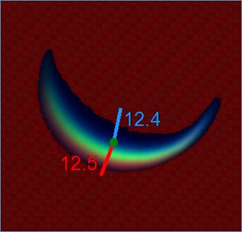
From this, notice the following :

· The background is shaded red – this is achieved by adjusting the Black Threshold control in the ADC Alignment panel (shown below). The red shaded area is ignored by SharpCap in its calculations, and you should adjust the Black Threshold so that all the dark area around the target is shaded, but avoid the shading covering any part of the target (including the colour fringes on its edges).

· The green dot shows the centre of brightness of the green channel of the image.

· The blue and red lines show how far (and in what direction) the centre of brightness of the blue and red channels are offset from the centre of the green channel. The length of the lines are increased to make them easier to see.

· The numbers adjacent to the lines show the size of the offset (in pixels) between the centres of the greed and red channel (in red) and the green and blue channel (in blue).

· In its simplest terms, the process of aligning the ADC is a matter of making adjustments to the rotation of the ADC and the magnitude of its correction to give the minimum possible values for the red and blue offsets.

A small number of controls are available to adjust the ADC alignment process:

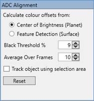
· Calculate colour offsets from – SharpCap can calculate the offsets between the colour channels in the image in two ways. For a planetary image, where the entire target is in the field of view, using the Center of Brightness option is appropriate. For images of a surface (lunar/solar) where the entire field of view is filled by the target, use the Feature Detection option instead. Feature Detection will automatically find image features in each of the three colour channels and calculate the position offsets between them.
Note that calculating offsets from surface feature detection is a SharpCap Pro feature.

· Black Threshold – this specifies the percentage image brightness that separates dark background (ignored) from bright target (included in calculations). Adjust this until the red shading covers all the background and surrounds (but does not cover) the target.

· Average Over Frames – How many frames of measurement will be taken before updating the graph with a new data point. If you have a noisy image you may want to increase this number.

· Reset – clear historical offset data from the graph.

· Track object using selection area – if you have used the Selection Area tool to restrict the measurements to a certain area of the image then you can check this box to have SharpCap automatically keep the selection area centred on the bright target within it (even if the target moves).

The Alignment history graph shows how the measurement of dispersion has changed over time (due to adjustments made to the ADC).

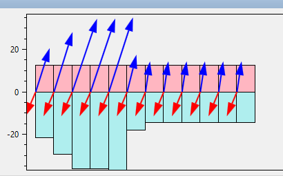
The length of the red line (red-green offset) on the display is tracked by the red columns shown above zero, while the length of the blue line (blue-green offset) is tracked by the blue columns shown below zero. The arrows show both the directions and relative lengths of each line at each measurement.

Newer measurements are continually added on the right hand side of the graph. Once the graph fills up, old measurements will gradually be moved off the left hand side allowing the latest data to be shown on the right.

Alignment Procedure

ADC Alignment is a two-step procedure, first getting the rotation of the ADC correct and then adjusting the amount of correction applied by the ADC to give the minimum possible values for the red and blue offset lines. You can read more about alignment procedure on the Sky Inspector ADC Page or try the procedure below.

Rotation Adjustment

For this stage, set your ADC to the maximum possible magnitude of correction. Once this is set and the ADC alignment tool in SharpCap is ready, gradually rotate the ADC (the camera can rotate too) through 360 degrees. Keep an eye on the size of the offset lines during the rotation. At one point in the rotation, the ADC will be pointing exactly in the wrong direction (180 degrees out) – at this point, the amount of dispersion and the length of the offset lines will be at a maximum, since the ADC and the atmosphere will both be acting to bend the colours in the same direction. At a point 180 degrees away from that maximum you should encounter a minimum value for the dispersion and the length of the offset lines – at this point the ADC is compensating for the atmospheric dispersion, but is over-correcting. Note that during this adjustment phase, the direction in which the offset lines point does not matter – you are only worried about the lengths of these lines and at which points in the rotation the lengths are largest and smallest.

Once you have located these two positions, position the ADC so that you are in the location which gives the smallest dispersion and is roughly opposite the largest dispersion point and move on to adjusting the magnitude of correction.

Magnitude Adjustment

This is a simpler adjustment stage – having completed the rotation adjustment above you know that the ADC is aligned in the correct direction, so it is simply a matter of gradually reducing the amount of correction that the ADC is applying until you get the minimum possible lengths of the two offset lines. Once this point is determined, you may wish to check to see if any small tweaks to the rotation help reduce the offsets further.

Collimation

SharpCap’s experimental collimation tool is designed to help spot collimation problems on Newtonian telescopes by measuring star size across the field of view.

If you take images of a well-focused star field with little nebulosity then in a correctly collimated Newtonian telescope the sharpest stars should be in the centre of the frame while stars towards the edges and particularly in the corners will be larger due to the effects of coma and (potentially) other aberrations.

When the collimation tool is activated, SharpCap will detect and measure the sizes of stars across the frame and highlight each detected star. SharpCap will also try to find a pattern in the sizes of stars across the frame and draw a contour plot of star sizes over the image.

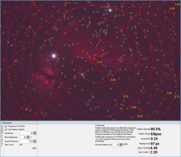
Small, well-focussed stars will be highlighted in green to yellow colours, larger, less well-focussed stars in orange to red colours. In the example above you can see that there is indeed an area with smaller stars surrounded by regions with less well-defined stars, but that centre of the pattern is just below the centre of the frame and is slightly elliptical rather than circular. This offset indicates that the collimation is not quite correct.

Offsets of the pattern from the centre are largely caused by incorrect collimation of the primary mirror. Elliptical patterns (i.e. non-circular) are largely caused by incorrect secondary collimation or camera tilt. A circular (or very nearly circular) pattern centred in the middle of the frame represents good collimation.

The normal Star Detection and other controls are available to the left-hand side – these are described in detail in the documentation on the Focus Tools Controls. The collimation tool additionally offers the ability to ignore star size variation on small spatial scales across the frame – sometimes this can help bring out the pattern of star size variation on the larger scale.

The collimation status information shows

· Pattern Strength – this is an indication of how much of the variation in star size is explained by the pattern. High strength patterns are more reliable than low strength patterns.

· Pattern Shape – this must be ‘Ellipse’ or ‘Circle’ for the tool to be useful – other patterns do not have a centre point and cannot be used to guide collimation

· Eccentricity – this shows how far from circular an elliptical pattern is. An eccentricity of zero means circular.

· Misalignment – this shows how far from the centre of the frame the centre of an elliptical or circular pattern is

· Max/Min FWHM – these figures show the minimum and maximum star widths measured in the frame

Note: while this tool can detect collimation errors, it can still be difficult to make adjustments successfully based on the measurements shown

Note: using a coma corrector dramatically reduces the coma of stars away from the centre of the field of view. While this improves images dramatically, it also makes it very hard or impossible for this tool to make accurate readings of collimation.